返回文章

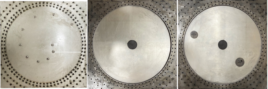
Figure 1.  Photograph of the niobium lid (left) and the basin of the MB which is formed by a 5-mm thick lead-coated brass plate with a circular hole of radius R = 250 mm on top of a niobium plate. The cavity MB1 contains a ferrite disk of radius R₀ = 30 mm at its center, mimicking a ring QB (middle) and additional lead-coated metallic disks for the cavity MB2 (right) in the experiments modelig a QB with mixed regular-chaotic dynamics.

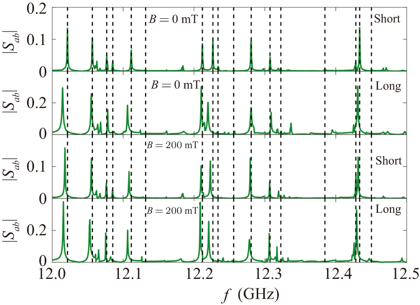
Figure 2.  Comparisons of the transmission spectra of the MB1 measured with short (first and third row) and long (second and fourth row) antennas at ≈ 5 K for external magnetic field B = 0 mT (first two rows) and B = 200 mT (last two rows). The black dashed vertical lines indicate the positions of the resonances of the MB1 with short antennas to facilitate the comparison with the other spectra.

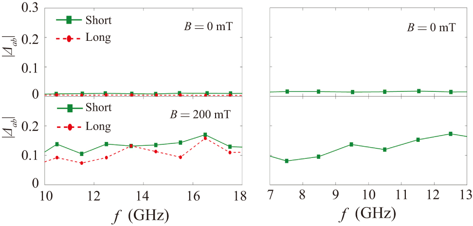
Figure 3.  Left: Relative size of the violation of the principle of detailed balance in the MB1 with short antennas (green squares) and long antennas (red dots) for B = 0 mT (top) and B = 200 mT (bottom). Right: Same as left panels for the MB2. Note that the symbols show the average values determined in 1 GHz windows.

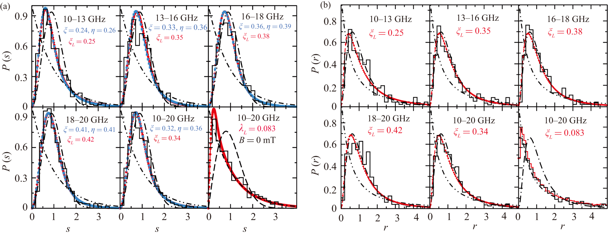
Figure 4.  (a) Nearest-neighbor spacing distributions. Shown are the experimental results for the MB1 for short antennas with B = 0 mT and B = 200 mT (black histograms). The red curves are obtained from a fit of the Wigner-surmise Eqs. (B1) and (B2) of the appendix to the experimental results with B = 0 mT and B = 200 mT, respectively, whereas the blue curves result from a fit of the Wigner-surmise Eq. (3). Shown are the results for 231 f_n ∈ [10,13] GHz, 294 f_n ∈ [13,16] GHz, 232 f_n ∈ [16,18] GHz, and 256 f_n ∈ [18,20] GHz, and for the whole considered frequency range, f_n ∈ [10,20] GHz. (b) Validation of the analytical result for the ratio distribution P^{1 → 2}(r) given in Eq. (C1). Here, we used the values of ξ_L determined from the fits shown in the left panel. The dash–dot–dot, dashed and dash–dotted lines show the corresponding curves for Poisson, GOE and GUE statistics, respectively.

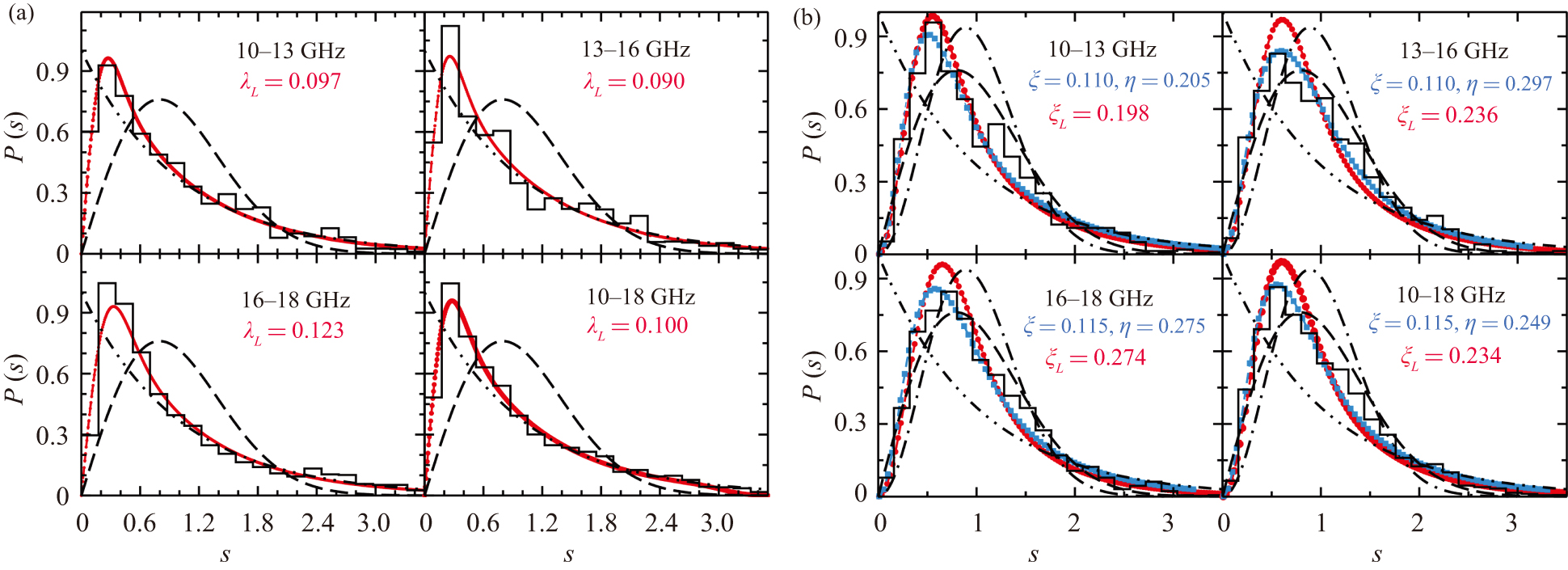
Figure 5.  Nearest-neighbor spacing distributions. Shown are the experimental results for the MB1 (black histograms) with long antennas for B = 0 mT (a) and B = 200 mT (b). Here, we chose the frequency intervals such that each of them contained 257 eigenfrequencies. The red curves are obtained from a fit of the Wigner-surmise Eqs. (B1) (left) and (B2) (right) to the experimental results, whereas the blue curves result from a fit of the Wigner-surmise Eq. (3). The dash–dot–dot, dashed and dash–dotted lines show the corresponding curves for Poisson, GOE, and GUE statistics, respectively.

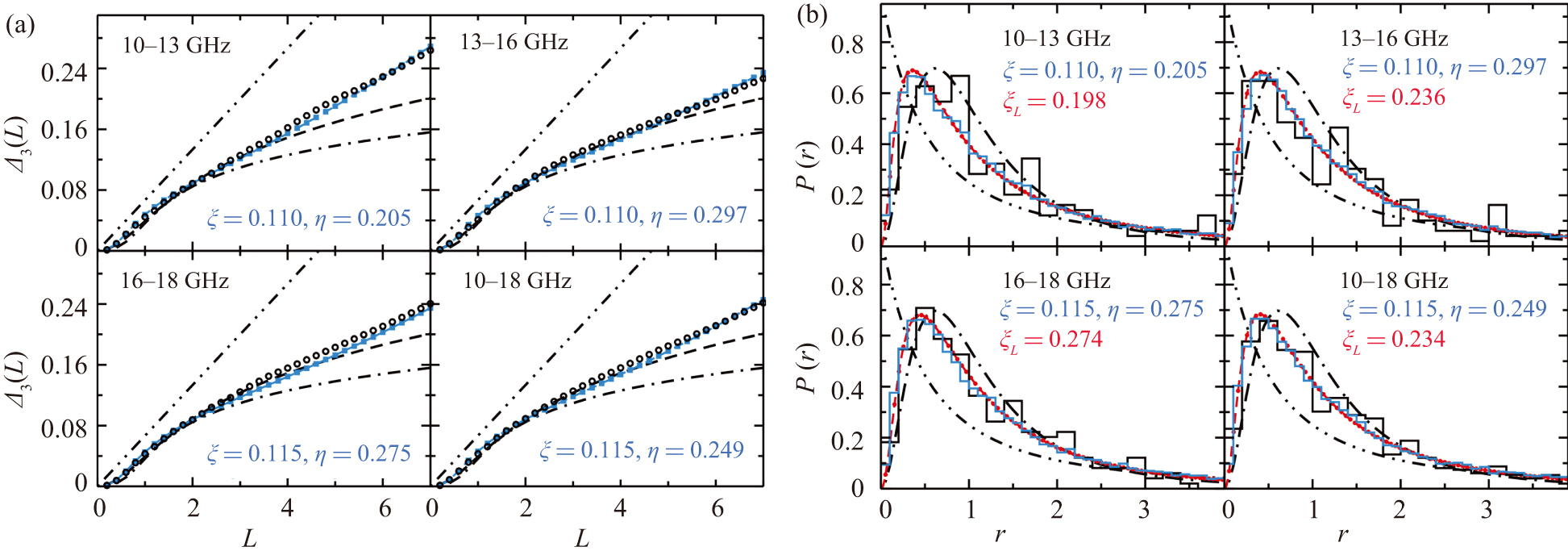
Figure 6.  (a) Dyson–Mehta statistics and (b) ratio distributions. Shown are the experimental results for the MB1 with long antennas (black circles and black histograms). The blue curves and red dots are obtained from an ensemble of random matrices of the form Eq. (2) and from Eq. (C1) using the values of ξ, η, and ξ_L, respectively, obtained from the fits in Fig. 5. The dash–dot–dot, dashed- and dash–dotted lines show the corresponding curves for Poisson, GOE, and GUE statistics, respectively.

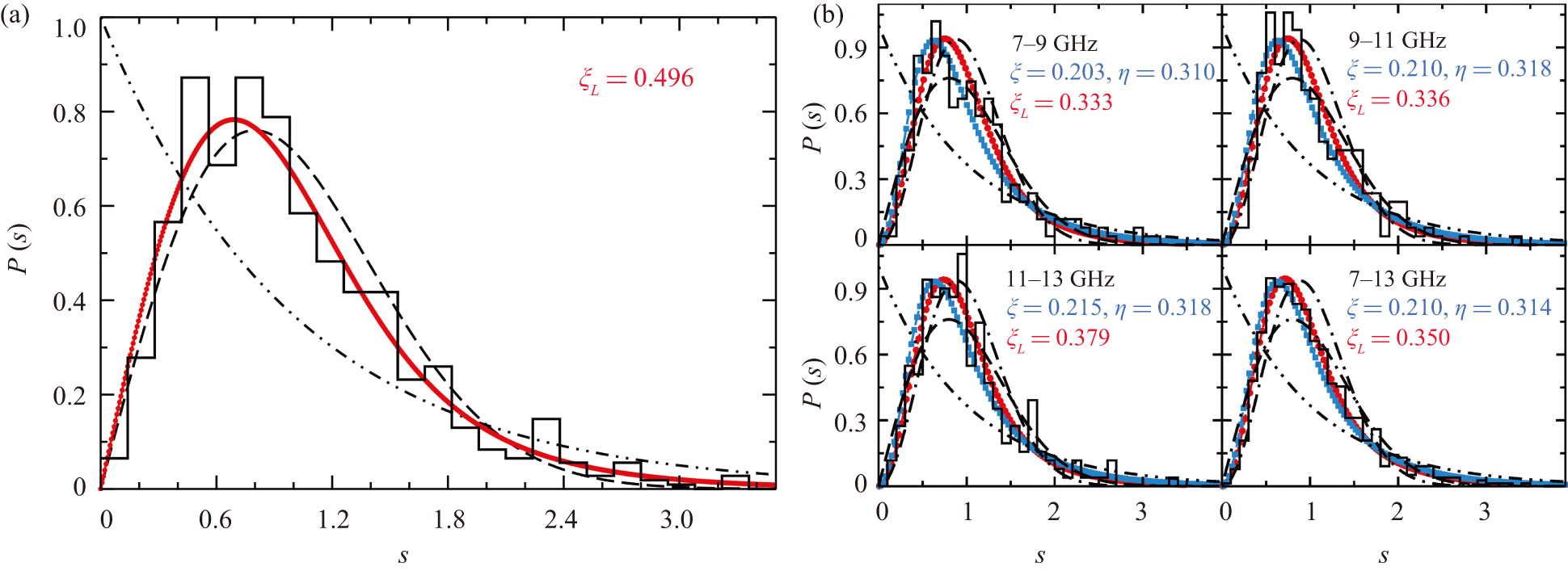
Figure 7.  Same as Fig. 5 but for the MB2.

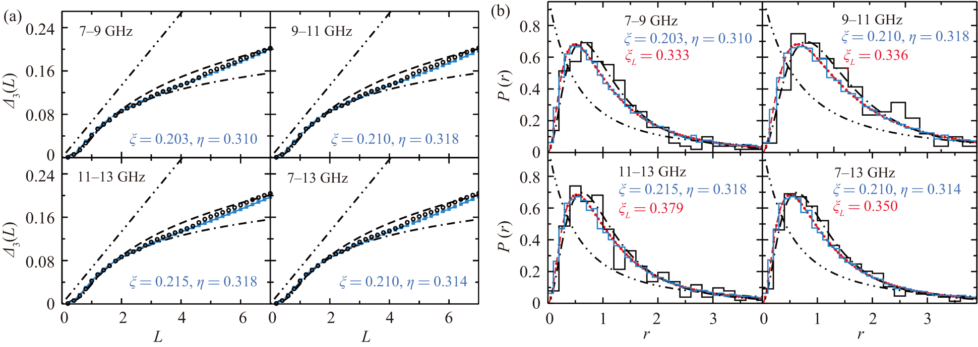
Figure 8.  Same as Fig. 6 but for the MB2.

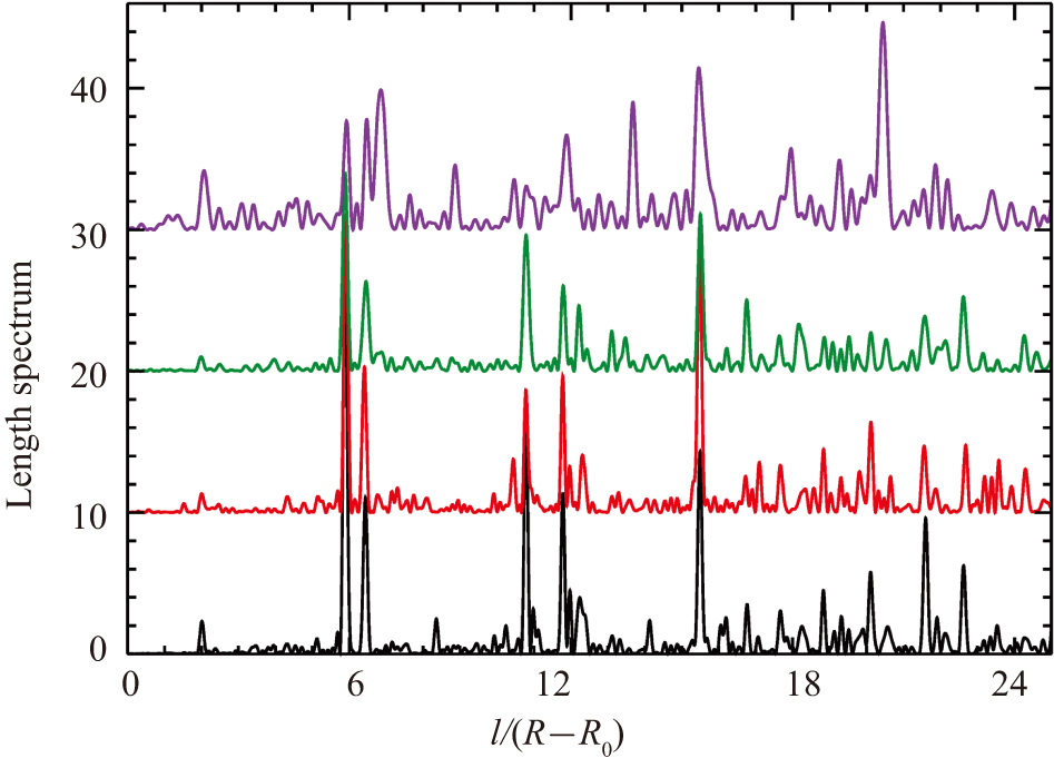
Figure A1.  Length spectra for B = 0 mT for, from bottom to top, the ring QB (black solid line), the MB1 for short (red solid line) and long (green solid lines) antennas, and the MB2 (violet solid line). Here, R = 250 mm denotes the radius of the circle billiard and R₀ = 30 mm the radius of the ferrite disk at its center. At lengths corresponding to orbits, that hit the ferrite disk and thus feel the differing BCs, the length spectra of the MB1 with short and long antennas differ.^[54]