-
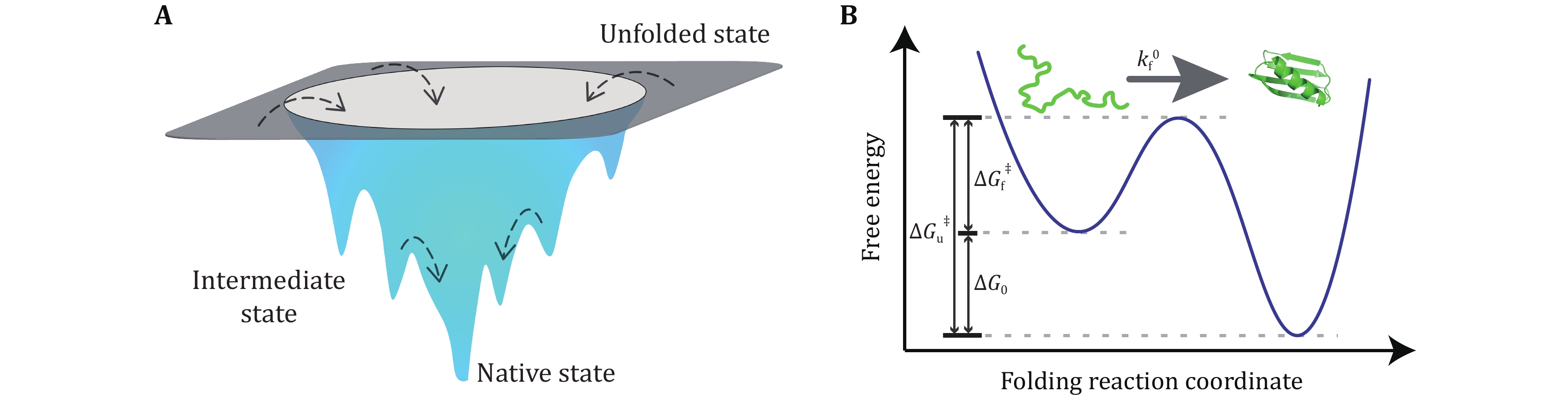
Figure 1. Schematic diagram of free energy landscapes in three-dimensional space and along a single reaction coordinate. A Schematic funnel-shaped energy landscape of a protein. The unfolded state of a protein has a large number of microscopic conformations, while the native state has a well-defined single conformation with minimal free energy. Multiple transition states may coexist between the unfolded and folded states (Bryngelson et al. 1995; Wolynes et al. 1995). B Typical free-energy profile of the free energy landscape of a two-state protein. The protein travels from the unfolded state through a transition state to its native state at a folding rate kf0. The free energy difference between the unfolded and folded states, ∆G0, defines the thermodynamic stability of a protein. The folding barrier ∆Gf‡ and the unfolding barrier ∆Gu‡ determine the folding rate and unfolding rate, respectively
-
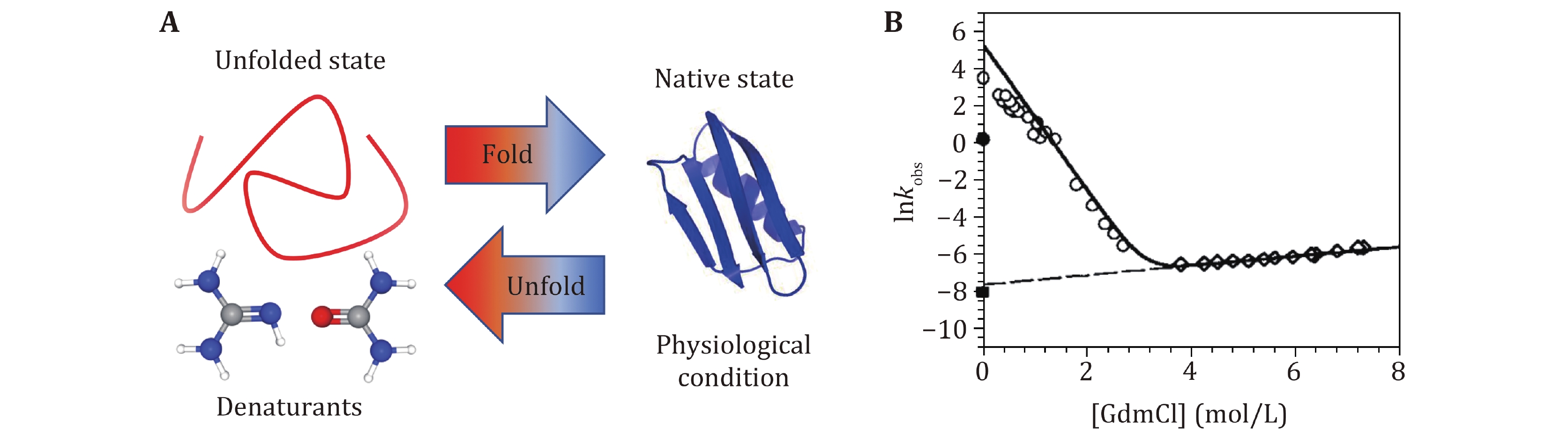
Figure 2. Biochemical technique to study protein folding and unfolding dynamics with denaturants. A Sketch of protein denaturation induced by denaturants. Proteins stay at unfolded state in high concentration denaturants solution, and at native state in physiological solution. B The typical experimental results of the observed relaxation rate as a function of the concentration of GdmCl. Reprinted with permission from the National Academy of Sciences (Carrion-Vazquez et al. 1999)
-
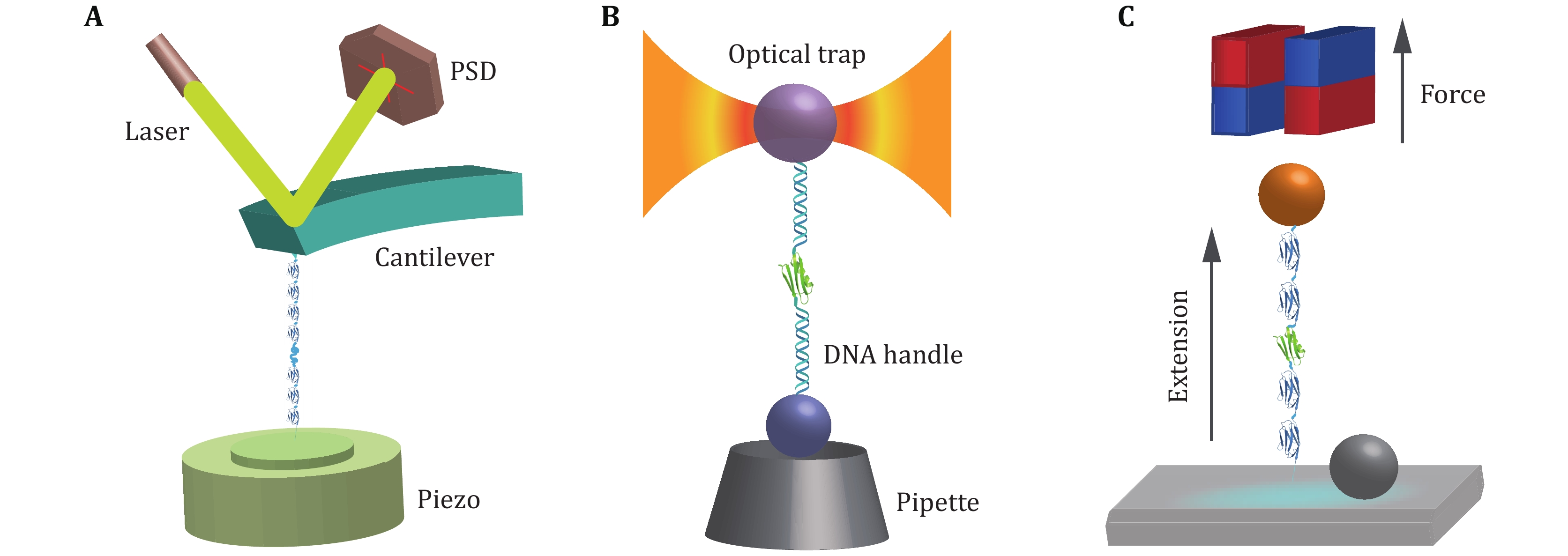
Figure 3. Cartoon schematics of SMFS techniques. A AFM: the poly-protein with repeating protein domains is tethered between the cantilever tip and the substrate surface. The retraction of the piezo stage in the axial direction increases the distance between the cantilever and the substrate to stretch the protein, and the force is measured from the deflection of the cantilever. B OT: the target protein is linked between a microsphere in the optical trap and another microsphere held by the micropipette via two DNA handles. Controlling the displacement of the microsphere in the optical trap, the force applied to the target protein and the extension changes can be recorded. C MT: the protein of interest is attached between a superparamagnetic bead and cover glass surface. A pair of permanent magnets located over the sample chamber imposes a constant force on the protein, while the extension is measured through real time analysis of the microscopic bead images
-
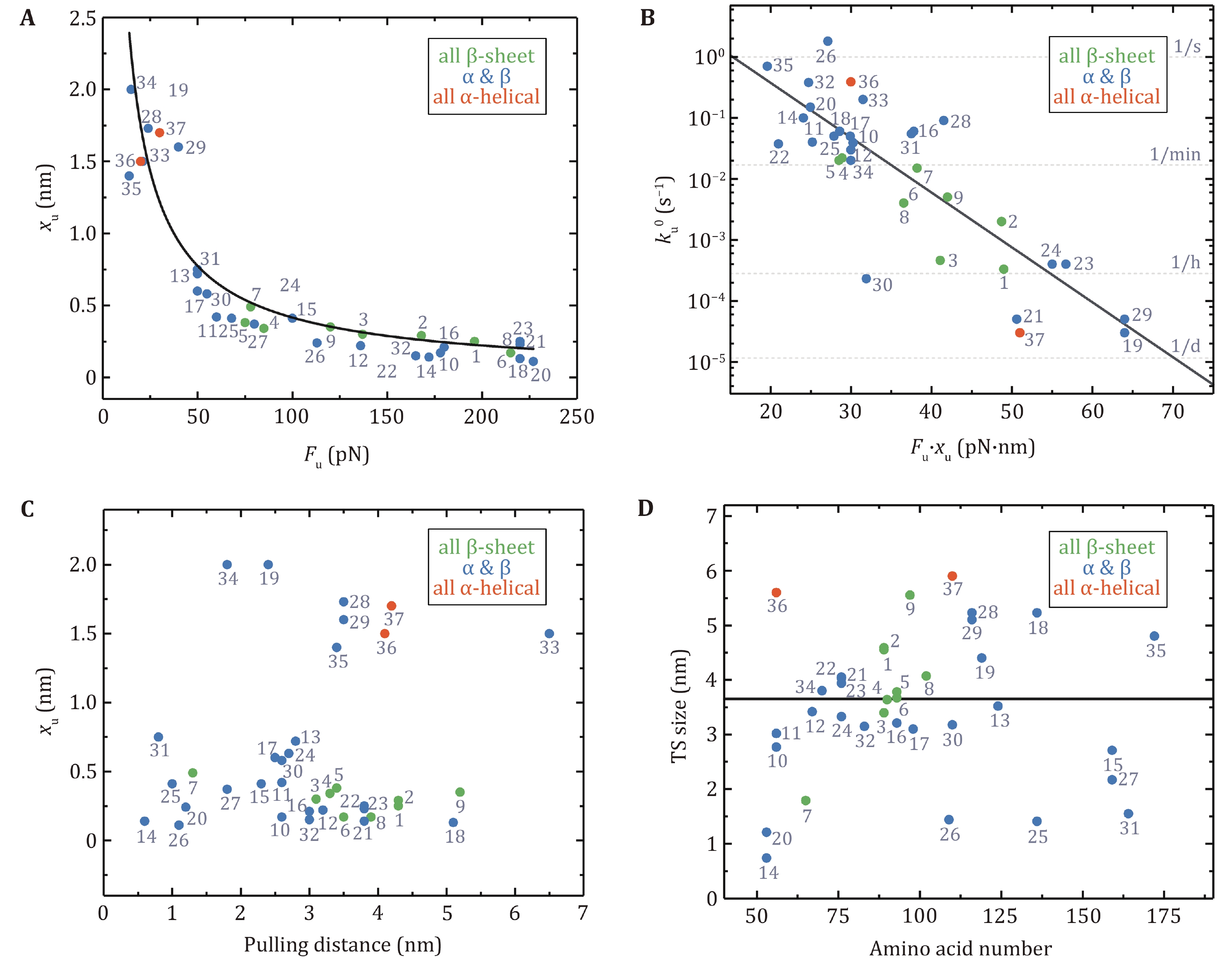
Figure 4. The relationships of mechanical properties of proteins in Table 1 obtained by AFM. Protein numbering in all pictures is the same as in Table 1. A The relationship between unfolding distance (xu) and mean unfolding force (Fu) at a pulling speed of 400 nm/s. The data can be described by the Bell–Evans model (black solid line) for the most probable unfolding force Fu = (kBT/xu)ln[r · xu/(ku0 · kBT)] using a fixed loading rate (r = 200 pN/s) and unfolding rate at zero force (
ku0 = 0.2 s−1) (Leblanc et al. 2021). B The dependence of the unfolding rate at zero force (ku0) on the product of the unfolding force and the unfolding distance (Fu · xu). Proteins with a high value of Fu · xu unfold several orders of magnitude more slowly than proteins with a low value of Fu · xu. The linear fitting has R2 of 0.70. C xu is plotted against the pulling distance. D The transition state size is plotted as a function of the number of amino acids in each protein. The black solid line is the average transition state size: 3.7 ± 1.5 nm (mean ± SD) -
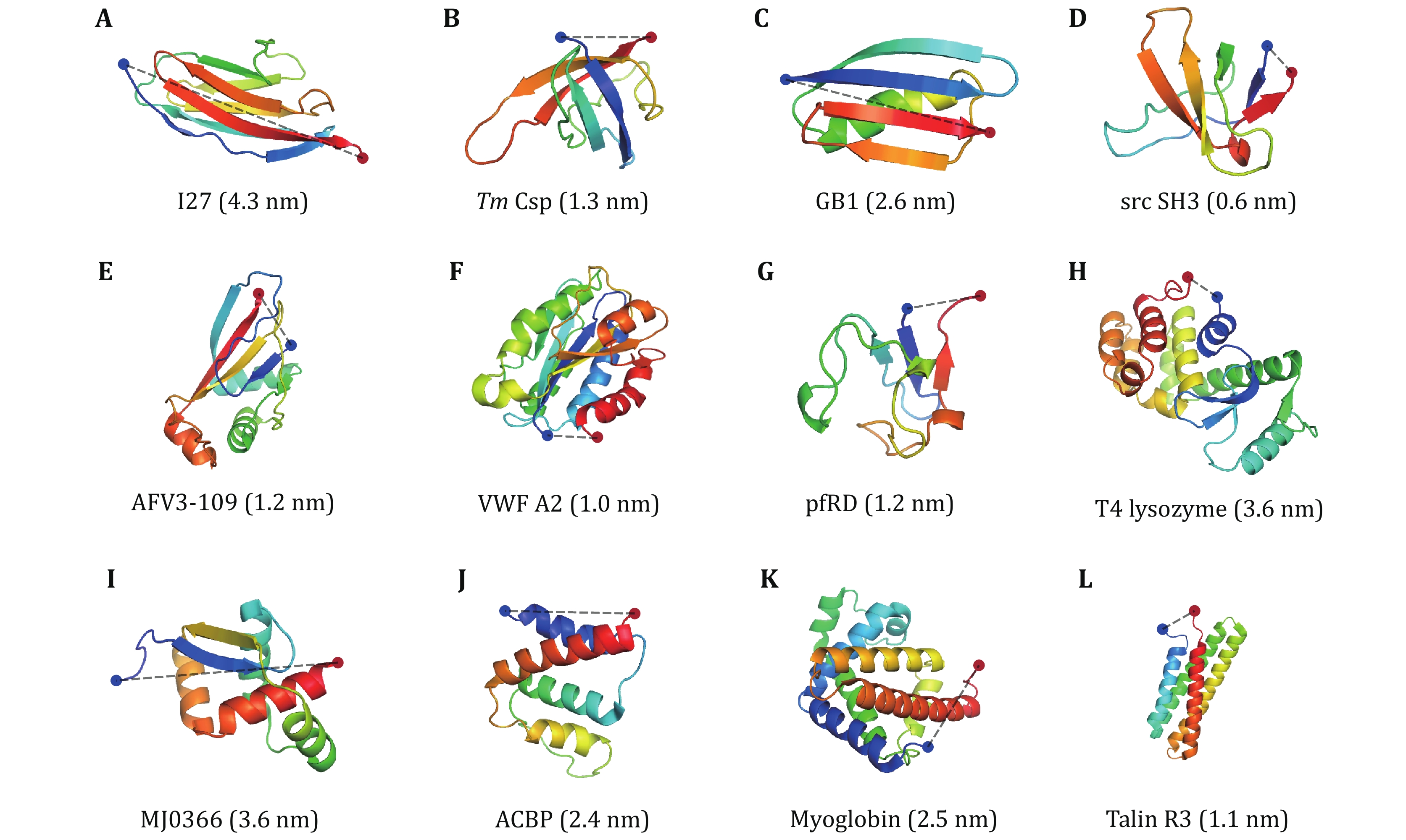
Figure 5. Three-dimensional cartoon representations of the native structure of all proteins studied by OT and MT (Table 2). The blue and red dots indicate the N- and C-termini of the protein, respectively. The N–C distances are given in parentheses. NuG2 is a computationally designed variant of the protein GB1, whose structure is not shown here
-
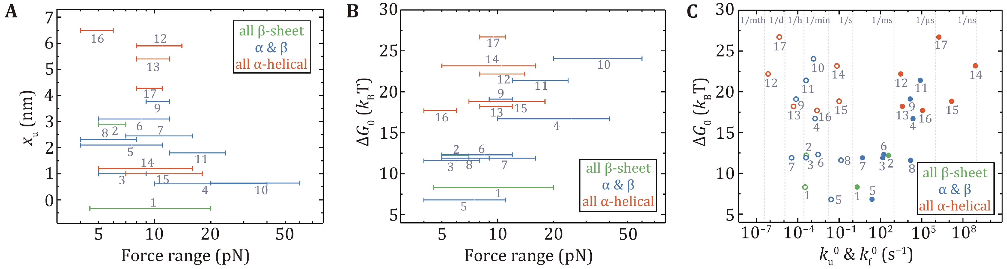
Figure 6. The relationships of mechanical properties of proteins in Table 2 obtained by OT and MT. Unfolding distance xu (A) and folding free energy ΔG0 (B) are plotted as a function of the experimental force range. C Correlation between ΔG0 and zero-force folding rates (solid circles), and correlation between ΔG0 and zero-force unfolding rates (open circles). Protein numbering in all the figures is the same as in Table 2
-
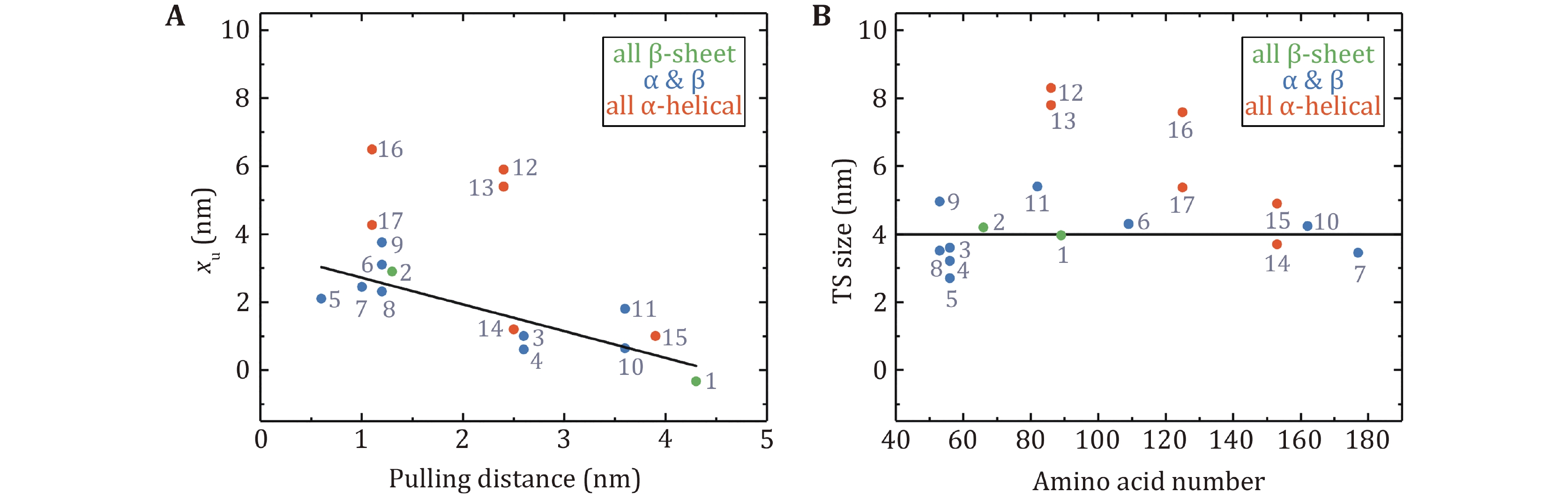
Figure 7. Unfolding distances and size of transition states obtained at low force by OT and MT. A The unfolding distance (xu) plotted as a function of the pulling distance. The linear fitting for proteins with β-strands has an R2 = 0.68. B The transition state size for proteins with different amino acid numbers. The black solid line is the average transition state size of proteins with β-strands: 4.0 ± 0.8 nm (mean ± SD). Protein numbering in both figures is the same as in Table 2
-
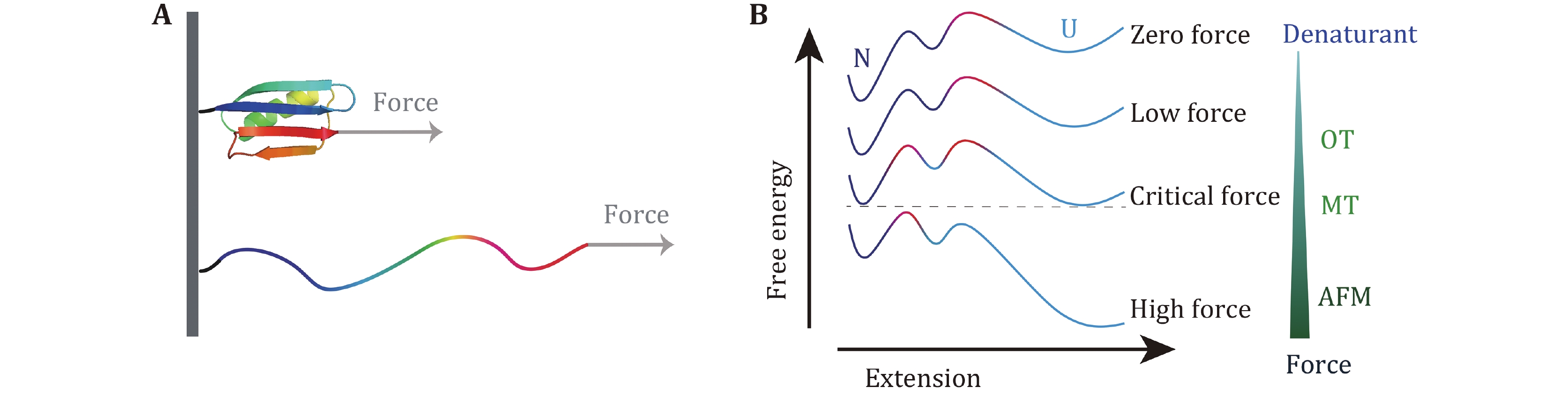
Figure 8. Detailed protein free energy landscape revealed by SMFS measurement over large force range. A Sketch of protein unfolding under stretching force. B Free energy landscape with two barriers and an intermediate at different forces. Red color part shows the dominant barrier with the highest free energy. At high force, only the barrier close to the native state can be detected, while at low force, additional information of the free energy landscape over larger conformational space can be studied
Figure
8 ,Table
2 个