返回文章

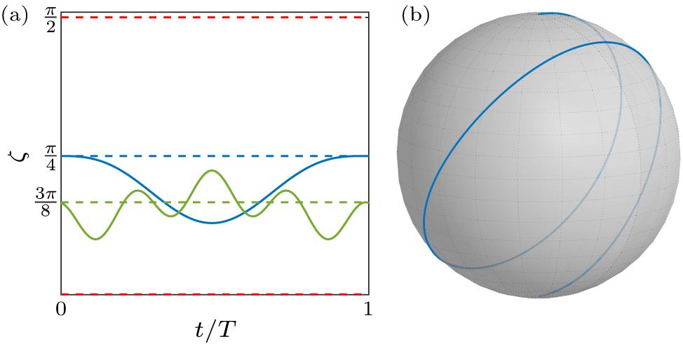
Figure 1.  Examples for σ_z control. (a) The different types of evolution with respect to the ζ(t) function. The start and final points of the evolution time are labeled as t = 0 and t = T, respectively. The red dashed line describes the limitation of ζ(t), which is set by the divergence of function cot[2ζ(t)]. The blue solid line describes an example of population exchange gate. The blue dashed line with unchanged ζ(t) = π/4 will reduce to Rabi oscillation with constant Rabi frequency. The green solid describes an example of rotations around the axis π/4 in the x–y plane, and the green dashed line with unchanged ζ(t) implements a rotation around the axis x + z with constant Hamiltonian when φ = 0. (b) The evolution path of the blue solid line in (a), where the population changes from the initial state |0〉 to the final state |1〉 in the Bloch sphere, leading to a NOT gate with the parameters being Δ = 2π MHz and T = 0.69 μs.

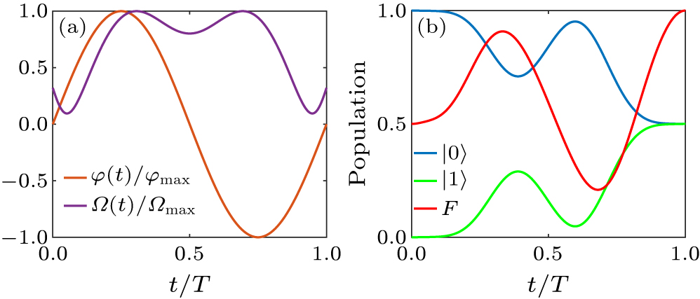
Figure 2.  An example of implementing H gate with σ_x/y control. (a) The time dependence of the Hamiltonian parameters, including the amplitude Ω(t) and phase φ(t) of the external driving field. (b) The fidelity and the qubit-state population dynamics for the H gate.

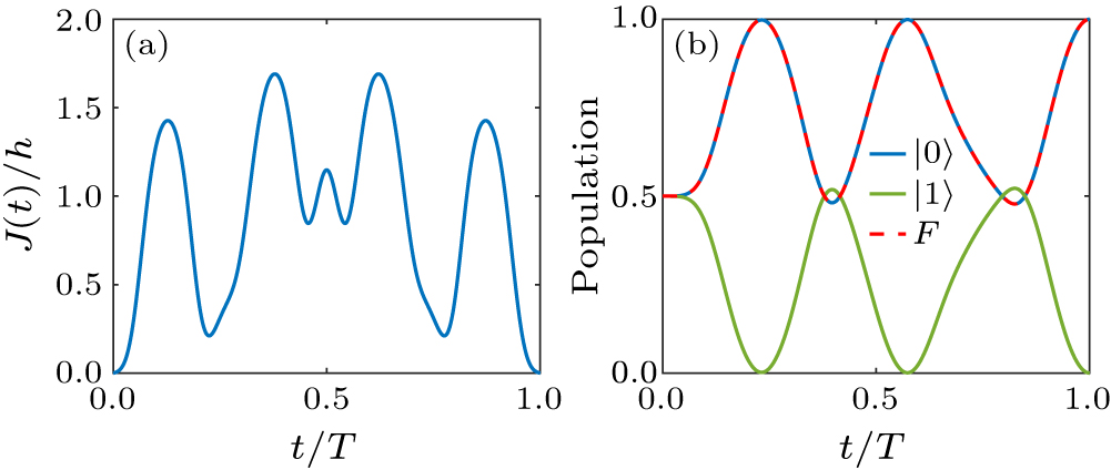
Figure 3.  (a) The pulse shape of J(t) to implement Hadamard gate with a smooth curve. The parameters are h/2 = 2π MHz and T = 0.942 μs. (b) Population of qubit states |0〉 and |1〉 and the corresponding gate fidelity in implementing the Hadamard gate.

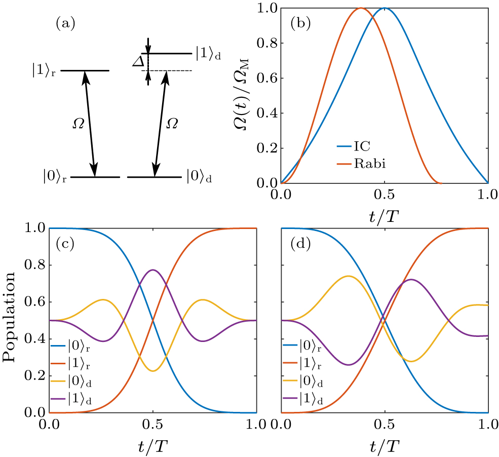
Figure 4.  Illustration of the example of individual control in a multilevel quantum system. (a) The energy level structure shows the scenario where the control pulse will also address the two-level subsystem in a detuned way, when two transitions are closely spaced in frequency. The resonant driving of the target subspace affects nearby transitions, leading to leakage in the target quantum dynamics. (b) This panel compares the pulse shapes for individual control (IC) versus a general Rabi pulse in the form of the sine function, i.e., Ω_M sin(πt/T), where two pulses have the same maximum amplitude Ω_M, while T represents the evolution time for the individual control pulse. (c) The populations of both the resonant and detuned subspaces for individual control, with parameters Δ = 2π MHz, T = 0.95 μs and ζ(t) = π/8–0.29⋅sin³(π⋅t/T). Using an analytical-assisted solution, an accurate NOT operation is achieved without leakage to the nearby transition at the final time. (d) The populations of both resonant and detuning subspaces for the general Rabi pulse Ω_M sin(πt/T), with the same parameters as in (c). While a NOT gate is obtained, the leakage of the control pulse results in unwanted evolution in the nearby transition.