Exact quantum dynamics for two-level systems with time-dependent driving

The search for exact solutions to the time-dependent Schrödinger equation has garnered significant interest since the beginning of quantum mechanics. Today, it continues to play a crucial role in various quantum tasks that demand precise control. In particular, the exact evolution of a two-level system under external driving has attracted considerable attention, as it enables accurate qubit control in quantum information processing. Since a time-dependent Hamiltonian is non-commutative with respect to different times, achieving arbitrary target evolution for a qubit poses a significant challenge. Consequently, exact solutions are typically found only for specific cases, such as the Landau–Zener transition,^[1,2] Rabi problems,^[3] and quantum control using the hyperbolic secant pulse.^[4]

Currently, the pursuit of exact dynamics or time-dependent unitary evolutions continues to attract significant attention, as it fundamentally addresses the challenges associated with the lack of precise quantum control. This is particularly relevant in both theoretical research and the experimental realization of quantum control and quantum computation. The primary obstacles include the quench effect, leakage associated with control pulses, and crosstalk among qubits.^[5–9]

Recently, different schemes for exact quantum dynamics have been proposed.^[10–25] Notably, an exactly solvable model for a two-level quantum system under a single-axis driving field has been proposed,^[26] enabling the analytical design of certain types of quantum manipulations.^[27–30] However, analytical solutions for more general cases remain elusive. Besides, previous solutions also have limitations regarding systematic parameters; for instance, the initial conditions of the pulse shape complicate the design of the target evolution operators. Furthermore, obtaining exact dynamics becomes challenging when the driving pulse includes a time-dependent phase in its off-diagonal terms. These limitations hinder the extension of the method to large-scale or long-time quantum control.

Here, we present an analytically assisted scheme for a general time-dependent Hamiltonian of a qubit under driving, capable of generating nearly infinite analytical solutions for its arbitrary dynamics. An arbitrary target evolution under this non-commutative Hamiltonian can be achieved as long as the Hamiltonian can be expressed as a functional of a dimensionless auxiliary function. Notably, these solutions can reduce to well-known analytical solutions, such as those for Rabi problems and the Landau–Zener transition, with specific choices of the auxiliary functions.

Furthermore, we demonstrate the application of our solution in two typical problems. First, we achieve exact quantum dynamics with smooth pulses when manipulating a singlet–triplet (ST) qubit in semiconductor quantum dot systems,^[31] effectively avoiding the discontinuities in pulse shapes encountered in previous schemes. Second, we implement individual control in multi-level quantum systems with nearby transitions.^[5] Our analytically assisted solution allows for the design of the Rabi frequency without the constraint of pulse area, enabling us to achieve two desired evolutions in both subspaces with a single pulse. Thus, our scheme offers an analytical-based approach for precise quantum control.

The rest of this work is organized as follows. In Subsections 2.1 and 2.2, we present our scheme and its theoretical derivation in detail, focusing on two different control directions within the qubit Hamiltonian. Subsection 2.3 discusses specific applications and their corresponding analytical dynamics. Subsequently, in Section 3, we address two applications, i.e., tackling the quench problem in experiments and mitigating the leakage of control pulses in multi-level systems. Finally, Section 4 provides a brief conclusion of this work.

In this section, we present our scheme for exactly arbitrary dynamics of the qubit system under different driving directions.

It is well known that the dipole-interacting Hamiltonian for a two-level quantum system, under time-dependent driving and after applying the rotating wave approximation, can generally be expressed as (assuming ℏ = 1)

where Ω(t) and φ(t) label the amplitude and phase of the driven pulse, Δ(t) is the detuning between the frequency of the driven pulse and the energy frequency of a qubit. Its time evolution operator, respected to the unitary condition, can be written as

where |u₁₁|²+|u₂₁|² = 1.

The first thing we need to consider is how to analyze the entire evolution in the form of algebraic equations, as solving the matrix equations can be quite challenging. To address this, we first rotate the entire system into a specific representation, which yields the Schrödinger equation for the evolution operator as

where the transformation operator S(t) is defined as

Then, we will convert the matrix equations into algebraic equations for the elements of the evolution operator in Eq. (4). To begin, we will introduce their new definitions

Then, we rewrite the matrix form of the Schrödinger equation as two algebraic equations

where v˙11 and v˙21 label the time derivatives of v₁₁ and v₂₁, and α(t) is defined as α(t)=2∫0tΩ(t′)dt′−φ+π. Combining two equations in Eq. (6), once get (v˙11/v11)(v˙21/v21)=−Ω2.

Next, we separate this equation into two distinct equations as

where κ(t) is an unknown complex parameter introduced to satisfy the combined equation. Then, we obtain a general solution for v₁₁ and v₂₁ as

where α₁ and α₂ are constants. These constant phases arise from the derivation operation and are unknown yet.

Finally, we deal with these important parameters. Substituting Eq. (8) into Eq. (6), we can express α(t) in terms of κ(t) as

where θ = θ₁–θ₂. Since Δ and φ need to be real, α(t), defined in terms of them, also needs to be real. With this consideration, we can separate the complex function κ(t) into its real and imaginary parts, labeling them as κ_R(t) and κ_I(t). This allows us to separate the right side of Eq. (9) into its real and imaginary components. Furthermore, considering the restriction that α(t) is real, it ensures that the right side of Eq. (9) contains no imaginary terms. Thus, we get

Furthermore, we can obtain the derivative form of this equation as follows:

Generally, this parametric equation cannot be solved analytically. However, it is not necessary to do so if the goal is to obtain the evolution operator. By defining a dimensionless function χ(t)=∫0tΩ(t′)sinκI(t), we aim to establish the relationship between the Hamiltonian and its evolution operator by parameterizing them as functions of χ(t).

To achieve the above goal, we need to parameterize κ(t) as the function of χ(t). Since κ_I(t) has already parameterized by χ(t), we only need to deal with κ_R(t). This parameterize is achieved by treating Eq. (11) as a differential equation for κ_R(t) and κ_I(t). And, they are parameterized as

where C is an undetermined constant that comes from the integral operation of Eq. (11), which will be discussed and determined later. Since we have parameterized κ(t) as a function of χ, the relationship between the elements of the evolution operator and χ has already been established. Introducing ζ(t) = χ(t) + C for clarity, the elements of the evolution operator, u₁₁ and u₂₁, can be calculated and expressed as functions of ζ(t) as

where the parameter ξ±(t)=∫0tΩ1−ζ˙2/Ω2csc(2ζ)dt′±12arcsin(ζ˙/Ω). Notice that we do not need to apply the transformation S(t) again, as we have already obtained the original elements u₁₁ and u₂₁ necessary to construct the evolution operator. In the above derivation, we have used two identities, i.e., sinh[ln(−tanx)] = cot2x and sinh[ln(−tanx)]–exp[ln(−tanx)] = csc2x. Then, the evolution operator can be written as

where ξ±′(t)=ξ±+[θ±(φ+π)]/2. Next, we address the integral constant C. As an integral constant can be arbitrary, the function ζ(t) should allow a non-zero value when t = 0. However, this setting appears to conflict with the initial condition stipulated in Eq. (14), which requires ζ(0) = 0 to ensure that the evolution operator is the identity when t = 0. To resolve this contradiction, we modify the evolution operator to satisfy both the arbitrary choice of C and the initial condition. It is given by

Note that the uncertain phases θ₁ and θ₂ cancel each other out in the final evolution operator U(t). This is reasonable, as the final solution should not contain any unknown parameters.

Then, we will determine the corresponding Hamiltonian parameterized by χ(t). Recalling the definition of α(t), we could get Δ(t)=[α˙(t)+φ˙(t)]/2. Since α(t) has already been parameterized by ζ(t), Δ(t) can be rewritten as a parametric function of ζ(t) as follows:

Note that ζ(t) is limited to avoid the divergence of the terms 1−ζ˙2/Ω2 and cot(2ζ), leading to the restriction of its value within the range of (0, π/2), as shown in Fig. 1. Furthermore, this restriction will limit the evolution time to the order of 1/Ω. Note that ζ(t) serves as an auxiliary dimensionless function, whereas ζ˙(t) is connected to physical quantities which have the unit of frequency, such as Ω(t) and Δ(t) in Hamiltonian. As a result, we obtain a relationship that the evolution operator and time-dependent Hamiltonian are both dependent on ζ(t). Since the form of the ζ(t) function can be designed almost at will, it allows for the generation of arbitrary evolution operators. In other words, we can design arbitrary ζ(t) functions and then derive the corresponding Hamiltonian and its evolution operator as an analytical-assisted solution.

Controlling the transverse σ_z term typically requires more precise control over the frequency of the driving pulse, which is generally more challenging than controlling the longitudinal σ_x/y term. Hence, we present the analytical-assisted solution under σ_x/y control. In this case, to distinguish from Eq. (1), we denote the general Hamiltonian as

This Hamiltonian is indeed equivalent to the Hamiltonian in Eq. (1). The main difference between them lies in the controllable elements. In Eq. (1), we assume control over the σ_z components to achieve a universal gate set, a scenario commonly found in ST qubit systems.^[31–33] Conversely, the method of controlling over σ_x/y components to realize the universality is more prevalent in quantum computation systems.^[34–37] It is important to note that the solution we have obtained thus far only permits control over the σ_z components for implementing a universal gate set, while control over the σ_x/y components remains restricted. To address this, we introduce a transformation to convert this off-diagonal controllable Hamiltonian into a diagonal controllable one, which is solvable as shown in the previous subsection. The transformation is

then the Hamiltonian in Eq. (17) is changed to

Now, since Ω′(t) is arbitrary, comparing with the Hamiltonian in Eq. (1), the evolution operator can be obtained by treating (Ω′(t)+φ˙/2) as the new parameter of the σ_z term in Eq. (1). As a result, the evolution operator can be written as

where U′(t) is the evolution operator with respect to the Hamiltonian in Eq. (19), which can be obtained according to the σ_z control case. And, the controllable off diagonal part in Eq. (17) can be expressed as

with Δ′′=−Δ′(t)+12φ˙(t). Furthermore, this analytical quantum dynamics enables the use of phase modulation, in addition to the conventional amplitude shaping, in designing a target quantum control pulse.

As the final result, we write the evolution operator in Eq. (15),

where

with ξ±(t)=∫0tΩ1−ζ˙2/Ω2csc(2ζ)dt′±12arcsin(ζ˙/Ω). Note that, the dynamics of evolution seems to depend on various parameters, but, will ultimately depend on one time-dependent term, the auxiliary function ζ(t). All of the other parameters, whatever in the form of Hamiltonian or evolution operator, can be written as the functional of auxiliary function ζ(t), for example, the parameter ξ(t), which depends on the integral and the derivative of ζ(t). Although the function ζ(t) itself has no direct physical significance, it serves as a crucial auxiliary function, capable of parameterizing other physical quantities. For instance, its time derivative, ζ˙(t), is related to physical quantities with units of T⁻¹, such as Ω(t) and Δ(t) in the Hamiltonian. Consequently, an almost infinite number of analytical solutions can be derived, as the auxiliary function ζ(t) can be set nearly arbitrarily, provided it remains within the valid range of (0,π/2).

Then, we will demonstrate that analytically-assisted solutions can reduce to the well-known analytical solutions of the Schdöinger equation. The dynamics for Landau–Zener transition, such as a ground state is driven through the anti-crossing produced by σ_x and ultimately returns with probability 1, could be reproduced. In the analytical-assisted solution, considering a ground state at t = 0, the probability for the system to be in the ground state at other time can be calculated by Eq. (15), i.e., |U₁₁(t)|². If we choose the auxiliary function ζ(t) to meet the condition ζ˙(0)=ζ˙(T)=0, the probability for the system in the ground state will be |e²ⁱξ₊cos[ζ(0)]cos[ζ(T)]+sin[ζ(0)]sin[ζ(T)]|², where T labels the evolution time. If we further ensure ζ(0) = ζ(T) = 0, a Landau–Zener transition solution can be reproduced. The Hamiltonian also indicates it since ζ = 0 will lead to an infinity value of σ_z according to Eq. (16), which satisfies the condition of Landau–Zener transition σ_z≫σ_x. Besides, the Rabi oscillation or other dynamics of time-independent Hamiltonian can also be reproduced if we set the auxiliary function ζ(t) to be time-independent. For example, a constant ζ = π/4 will lead to a Rabi oscillation while the parameter ξ(t) in Eq. (14) becomes the integral of Ω(t).

Therefore, as a direct application of the solutions, considering an uncontrollable and inevitable time-dependent or time-independent function in the σ_x/y/z part, achieving a desired two-level evolution can still be accomplished through the analytical-assisted solutions. For instance, if the σ_z part of the Hamiltonian contains an uncontrollable and time-dependent term Δ(t), it is still possible to derive the desired evolution operator as in Eq. (15) by designing only one function, ζ(t). Further, the Hamiltonian in other part is also determined since they depend on ζ(t) and Δ(t) according to Eq. (16). Moreover, we show more examples with different ζ(t). It is worth noting that different choices of the parameter ζ(t) lead to various evolution operators. However, the most common types of evolution operators can typically be obtained under the simpler condition ζ(0) = ζ(t), which makes it easier to determine and calculate other parameters. Thus, we set ζ(0) = ζ(t) and express ζ(0) using a trigonometric series for convenience. Specifically, we set

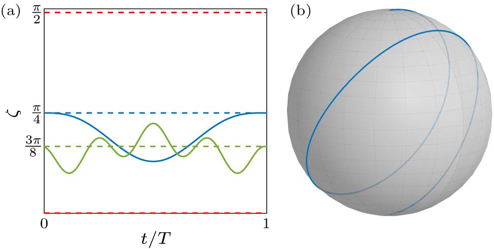
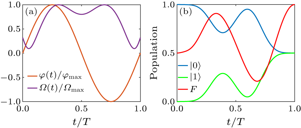
where A_n is a constant, and the trigonometric series are involved to satisfy ζ(0) = ζ(t). Two examples are shown in Fig. 1, with the boundary conditions of ζ(t) to respect population exchange gates and Hadamard like gates, with parameter sets of {A₀,A₁,A₂,A₃} = {π/4, 0, 0, −0.38} and {A₀, A₁, A₂, a₂, A₃, a₃} = {3π/8, 0, −0.22, 4, 0.18, 1}, respectively. And the ζ(t) function is plotted in Fig. 1(a). In Fig. 1(b), we show an evolution path of the NOT gate by further setting Δ = 2π MHz and T = 0.69 μs. Similar to σ_xy control, we design a Hadamard gate when assuming there exists a harmful constant detuning Δ′ = 2π MHz and the time-dependent phase φ(t) = sin(2πt/T), as shown in Fig. 2. The Hadamard gate can be obtain when the parameters of ζ(t) are {A₀, A₁, a₁} = {π/8, 0.26, 1} and time T = 0.66 μs. The fidelity of the state |ψ(t)〉 is defined as F(t) = |〈Ψ|ψ(t)〉|², where |Ψ〉 labels the ideal target state.

In this section, we demonstrate that the analytical solution can be utilized to implement universal gates with smooth pulses, which are well-suited for experimental setups.

The Hamiltonian for ST qubit in semiconductor double quantum dot systems^[31–33] is

with the qubit basis |0〉=|T〉=(|↑↓〉+|↓↑〉)/2 and |1〉=|S〉=(|↑↓〉−|↓↑〉)/2, where |↑〉/|↓〉 indicates the spin up/down of an existed electron in left or right dot. h = gμΔB_z and J(t) is the exchange interaction of two dots. Considering the randomized benchmarking (RB)^[38–40] would choose different quantum gates randomly in the Clifford gate series to test the quality of gate implementation, these 24 Clifford gates^[41] need to be implemented by the Hamiltonian Eq. (25). In the single-transmon (ST) qubit system, the Hamiltonian comprises only the σ_x and σ_z terms, which are used for implementing quantum gates. Typically, the value in the σ_x term remains time-independent. Previously, to implement quantum gates, it was necessary to keep the time-dependent parameter J(t) constant throughout the evolution, as the dynamics could not be solved if J(t) is time-dependent. Therefore, this manipulation can result in unwanted discontinuities in the pulse profile at the beginning and end of each gate when RB is performed. These discontinuities can lead to infidelities in the RB process, as it is challenging to achieve the exact realization in experiments. Therefore, we prefer smooth pulse schemes without such breaking points.

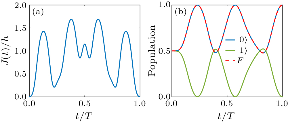
We demonstrate that the smooth pulses can be achieved using the analytical-assisted solution. The Hamiltonian in Eqs. (25) and (16) suggests that the time-dependent σ_z control scheme is suitable for the ST qubit system. Since h is time-independent and φ = 0, we obtain the expression of J(t) as a functional of ζ(t) as

Note that, the evolution operator in Eq. (14) does not depend on ζ¨(t) directly. Therefore, it is possible to design the suitable ζ¨(0) and ζ¨(T) to ensure that the value of J(t) at the start and end points can be a fixed constant (usually zero) in the implementation of all the 24 Clifford gate operations. As a result, a RB process with smooth pulse is obtained.

As demonstrations, we show how to construct Hadamard (H) gate and S gate, which are the generators of the group of 24 Clifford gate operations. To achieve smooth pulses, we set the value of the time-dependent J(t) to be zero at the start and end points for both gates. For the H gate, the π rotation around the x + z axis, we choose the boundary condition of ζ(0) = ζ(t) = 3π/8, numerically solve the equations to ensure ξ_± = π/2. As a specific example, we choose the trigonometric series of ζ(t) in Eq. (24) as

with parameters {A₀, A₁, A₂, a₂, A₃, a₃} = {3π/8, 0, −0.22, 4, 0.18, 1}. Under these settings, a H gate is implemented. The pulse shape of J(t)/h, the corresponding state population and the gate-fidelity dynamics of this case are shown in Fig. 3.

Besides, to realize the S gate, or any other phase gates, the decomposition in the ST qubit system is

where R(σ_z/x,ξ) describes a rotation around axis σ_z/σ_x in the Bloch sphere. To obtain this phase gate, an arbitrary rotation around the axis σ_x is needed. According to Eq. (24), it could be realized by setting ζ(t) according to Eq. (24) as

The parameter ξ could be solved numerically to satisfy ξ = π/4 or ξ = π/8 to implement S or T gate, respectively. As an example, we could set the parameters {A₀,A₁,A₂,A₃,a₃} = {π/4,0,0,0.24,1} to perform R(σ_x,ξ = π/4). By combining this gate with two H gates, we obtain an S gate. Since the compositions of H and S gates can generate all 24 Clifford gates, any RB process can be realized using only smooth pulse gates.

In many quantum control systems, there are numerous nearby transitions with comparable frequencies. Consequently, when implementing a desired manipulation on a target transition, there will inevitably be leakage to nearby transitions with different detuning. This is also the case for some qubit systems, such as NV-center systems,^[34] trapped ions,^[35] and molecular systems.^[36] We here show an example of individual control over two nearby transitions by using our analytical-assisted solution, and the corresponding energy level structure is presented in Fig. 4(a). This driving Hamiltonian on both transitions could be written as

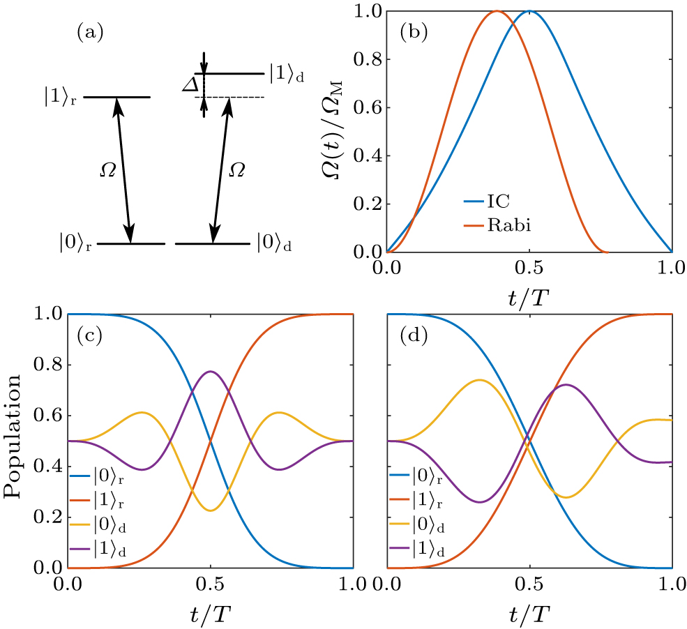
Furthermore, another application of our solution is the ability to achieve precise control over both the target subspace and the nearby subspace. This allows for using one pulse to control two subspaces individually. Specifically, in the target subspace, a resonant Rabi process is implemented by designing the Rabi rate Ω(t) and the phase φ. The integral area of ∫0TΩ(t)dt is then calculated to realize the desired quantum gates, where T labels the operation duration. This Rabi process with different phase φ could obtain universal control over the target resonant subspace. Notice the quantum gates in this resonant subspace do not restrict the pulse shape but only set the pulse integrals. Meanwhile, for the nearby detuned subspace, we can design the pulse shape to match the analytical-assisted solution and achieve universal quantum control over it, as long as we do not change the value of the pulse integral. As a result, an arbitrary individual control over two transitions can be obtained.

Now, we show the example to obtain individual controlling. The choice is ζ(0) = ζ(T) = π/4 with free φ(t), it can implement arbitrary phase gates, as shown in Fig. 1. The corresponding evolution operator is

Since the phase ξ depends on ζ(t), we can design ζ(t) to implement a desired phase gate. For example, an identity gate can be obtained when ξ = π. We show numeral simulations of the case, in which implementing an individual control consists of a NOT gate in the resonant subspace and a phase gate in the detuned subspace, described in Fig. 4. Moreover, for the situation φ = 0, another choice of ζ(t) can be used, it is ζ(0) = ζ(T) = π/6. It implements a rotation gate around the axis σ_x in the resonant subspace and a gate determined by the value of ξ in the nearby detuned subspace. The corresponding evolution operator is

If we design ζ(t) to satisfy ξ(T) = π and ensure ∫0TΩ(t)dt=π, we can realize an individual control gate consisting of a NOT gate in the resonant subspace and an identity gate in the detuned subspace. As is known, a direct square pulse implementing the same individual control gate requires Ω=Δ/3, which can be reproduced by this analytical solution case when setting ζ(t) = π/6 for the whole time.

In conclusion, we present an analytical-assisted solution of the time-dependent Schrödinger equation for a two-level quantum system under driving, with few limitations. We show the details of the analytical progress and present some concrete examples to demonstrate its application in quantum control, i.e., deriving smooth pulse for the gate operation in ST qubit systems and individual control over two transitions with nearby frequencies.

Further exploration in the field may be the following. First, this solution could also take the gate robustness into account by choosing different free parameters. Second, it is important to extend the study to higher-level systems, such as three-level systems, which can be used to model superconducting transmon qubits. This involves incorporating new operators specific to three-level systems and reproducing the theoretical derivations. Finally, the results presented here can also be extended to open quantum systems. By employing the Lindblad equation to simulate the density matrix, we ensure that the dynamics we obtain remain valid.