Experimental test of an extension of the Rosenzweig–Porter model to mixed integrable-chaotic systems experiencing time-reversal invariance violation

The objective of quantum chaos^[1–3] is to identify signatures of classical chaos in the fluctuation properties of the eigenvalue spectrum and the features of the wave functions of the corresponding quantum system. Concerning the spectral properties of typical quantum systems two conjectures have been formulated. According to the Berry–Tabor conjecture,^[4] the eigenvalues of quantum systems with an integrable classical counterpart exhibit Poissonian statistics classified with β = 0. On the other hand, the Bohigas–Giannoni–Schmit conjecture^[5–7] states that the spectral properties of typical quantum systems, whose corresponding classical dynamics is fully chaotic, are described by the Wigner–Dyson (WD) ensembles of random matrix theory (RMT). If time-reversal (T) invariance is preserved, they are predicted to agree with those of random matrices from the Gaussian orthogonal ensemble (GOE) with β = 1, if it is violated with those of random matrices from the Gaussian unitary ensemble (GUE) with β = 2.^[3,8] Indeed, in the past four decades RMT was successfully applied to analyze aspects of single-particle and many-body quantum chaos.^{[1–3,9–19]} Originally, it was introduced by Wigner, who was the first to propose that there is a connection between their spectral properties and those of random matrices,^[20–22] to describe properties of the eigenstates of complex many-body quantum systems like nuclei.^{[9,10,12,14,18,23]} A paradigm model for the verification of the conjectures and the study of aspects of quantum chaos are quantum billiards (QBs) whose classical counterpart are two-dimensional billiards (CBs).^[24–28] These consist of a bounded two-dimensional, simply-connected domain, in which a pointlike particle moves freely and is reflected specularly at the boundary, and their dynamics depends only on the shape of the billiard. Numerous theoretical^[1,3] and also experimental studies have been performed in the context of quantum chaos with microwave billiards (MBs) modeling QBs^[29–35] and with microwave graphs modeling quantum graphs.^[36–46]

Also, for typical systems with mixed regular-chaotic dynamics RMT models have been developed that interpolate between Poisson and WD statistics, for example the RP model^[47–51] and the β ensembles for general β.^[52,53] In Ref. [54] we investigated experimentally with a circular MB the properties of typical quantum systems undergoing a transition from Poisson to GUE statistics and validated analytical results for the corresponding RP model. An MB is a flat, cylindrical microwave resonator,^{[30,32,34,55]} which is operated with microwaves whose frequencies are below the cutoff frequency f^cut of the first transverse-electric mode. In that frequency range the associated Helmholtz equation is scalar and mathematically identical to the Schrödinger equation of the QB of the corresponding shape with Dirichlet boundary conditions (BCs). For typical T-invariant systems with chaotic classical counterpart complete sequences of several 1000 eigenfrequencies^[35,56,57] were obtained at liquid-helium temperature T_LHe = 4 K with niobium and lead-coated microwave resonators that become superconducting at T_c = 9.2 K and T_c = 7.2 K, respectively. Quantum systems with chaotic classical dynamics and partially violated T invariance^[58–62] were investigated experimentally in Refs. [63–65] and at room temperature in MBs.^{[33,36,39,40,66–70]} In these experiments, T invariance was violated by inserting a ferrite into the MB and magnetizing it with an external magnetic field B. This is not possible at superconducting conditions with a lead-coated cavity^[35] due to the Meissner–Ochsenfeld effect,^[71] because lead is a superconductor of type I.^[72] Accordingly, the top and bottom plates of the cavities used in Refs. [54,73] were made from niobium, which is a type-II^[74] superconductor for 153 mT ≤ B ≤ 268 mT, to realize MBs whose spectral properties undergo a transition from GOE to GUE, and from Poisson to GUE, respectively. The crucial advantage of superconducting MBs is, that complete sequences of about 1000 eigenfrequencies could be identified in these experiments, which would not be achievable with normal conducting MBs.

In this paper we present analytical and experimental results for the spectral properties of quantum systems with mixed regular-chaotic dynamics and preserved T invariance, that are subject to T-invariance violation. The measurements were performed with superconducting MBs employing the same procedure as in Ref. [73] to induce T-invariance violation. The basic MB has the shape of a ring billiard as in Ref. [54], and the transition from integrable to chaotic dynamics is realized by either using long antennas or inserting two circular disks, respectively. The objective is to develop a procedure for the determination of the size of chaoticity and of T-invariance violation. For this we employ an extension of the RP model,^[47] which is applicable to typical quantum systems experiencing a transition from Poisson to WD statistics, to one which is applicable when T-invariance violation is induced in a quantum system with mixed regular-chaotic classical dynamics. The RP model was intensively studied about 3–4 decades ago,^{[60,62,75–82]} and recently in the context of many-body quantum chaos and localization.^[83–95]

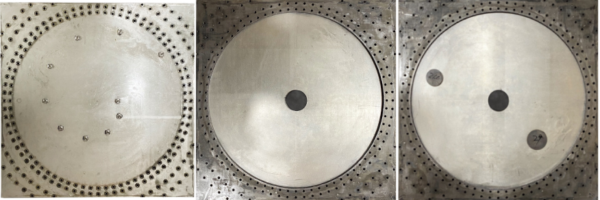
The experiments are performed at superconducting conditions with a circular MB with radius R = 250 mm which contains a ferrite disk with radius R₀ = 30 mm at its center. Photographs of the lid and basins of the MBs that were considered in this paper are shown in Fig. 1. As demonstrated in Ref. [54] the MB with just a ferrite at the center, referred to as MB1 in the following, emulates the spectral properties and length spectra of the corresponding ring QB, as illustrated in Fig. A1 in the Appendix A, implying that its classical dynamics is integrable. The cavity is constructed from three 5-mm thick plates, namely top and bottom niobium plates and a brass plate in between, which has a circular hole of radius R = 250 mm. The sidewall of the hole is coated with lead, and grooves were milled into the top and bottom surface of the middle plate along it. Furthermore, holes were milled out of all plates along circles; see Fig. 1. To realize a superconducting cavity with a high quality factor of Q ≳ 5 × 10⁴, the plates were screwed together tightly through these holes, tin-lead was filled into the grooves to attain a good electrical contact and the cavity was cooled down to below ≈ 5 K in a cryogenic chamber constructed by ULVAC Cryogenics in Kyoto, Japan. The cavity height, h = 5 mm, corresponds to a cutoff frequency f^cut = 30 GHz.

The height of the ferrite disk equals h, corresponding to a cutoff frequency fFcut≈4.5GHz and it is made of 19G3, whose saturation magnetization is M_s = 195 mT and niobium is a superconductor of type II^[74] as long as the magnetic field is chosen between two critical values, B_c1 = 153 mT and B_c2 = 268 mT. Namely, below B_c1 it behaves like a superconductor of type I and above B_c2 it becomes normal conducting.^[96] Thus the ferrite could be magnetized at superconducting conditions with a static magnetic field of strength B = 200 mT generated by two external NdFeB magnets, thereby achieving partial T-invariance violation at T_LHe and chaoticity.^[54] We demonstrated in Ref. [97] that the spectral properties of a circular cavity which is loaded with a magnetized ferrite material, agree above the cut-off frequency with those of a classically chaotic quantum system with a mirror symmetry and completely violated T invariance. Thus, the magnetized ferrite disk acts like a random potential.^[54]

In total 10 antenna ports were fixed to the lid. In the experiments emulating a ring QB, the lengths of the antennas were chosen such that they reached 0.5 mm into the cavity, to ensure that all resonances are excited, that the cavity has a high quality factor and that it is optimally closed. Note, that one long antenna suffices to change the spectral properties of an MB with the shape of a typical integrable CB from Poissonian to intermediate statistics. The long antenna is accounted for in the associated Helmholtz equation by a delta-function potential with a frequency-dependent amplitude, implying that the strength of the perturbation caused by it increases with frequency.^[98] Actually, it has been demonstrated in Refs. [98–101] that such MBs emulate singular billiards.^[102–107] Thus, to attain an MB modelig a QB whose classical dynamics is not singular, but integrable with a small chaotic part, we used 10 long antennas, that reached 2 mm into the cavity. To realize an MB, denoted as MB2 in the following, which simulates a QB with mixed regular-chaotic classical dynamics with a large chaotic part, we inserted two lead-coated copper disks with radii 24 mm and 29 mm into the MB1. Note, that in Ref. [108] we performed experiments with a large-scale circle-sector shaped MB which contained metallic disks, whose sizes were sufficiently small as compared to that of the MB, to model QBs with nearly-integrable classical dynamics, whereas in the present experiments the dynamics is clearly non-integrable, but not fully chaotic as in the case considered in Ref. [54].

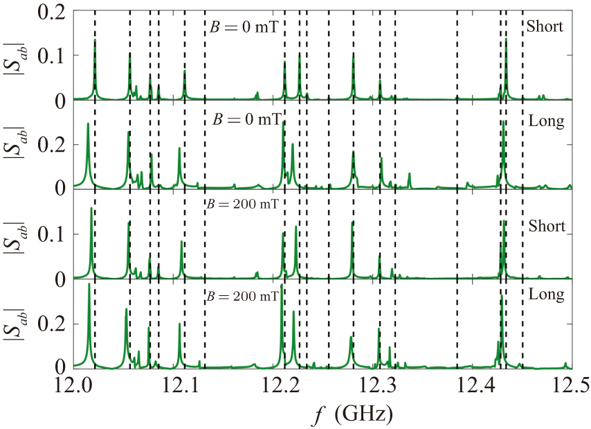
The positions of the resonances in the reflection and transmission spectra of a MB yield its eigenfrequencies f_n. They were measured by attaching antennas to the 10 ports and connecting them via a switch to a Keysight N5227A vector network analyzer (VNA) with Q086MMHF-0110CM-1L coaxial cables suitable for frequencies below 50 GHz. The VNA couples microwaves into the resonator via one antenna a and receives them at the same or another antenna b, and determines their relative amplitude |S_ba| and phase ϕ_ba, yielding the S-matrix elements, S_ba = |S_ba|e^iϕ_ba. In the measurements performed at superconducting conditions the resonances were isolated in the considered frequency ranges and thus well described by the complex Breit–Wigner form, Sba=δba−iγnaγnb/(f−fn+(i/2)Γn), with γ_na and γ_nb denoting the partial widths associated with antennas a and b and Γ_n the total resonance width, which is small since absorption into the walls of the MB is negligible at superconducting conditions. To identify the eigenfrequencies we fit the Breit–Wigner form to the resonances and thereby obtained complete sequences for both cavities for B = 0 mT and B = 200 mT.

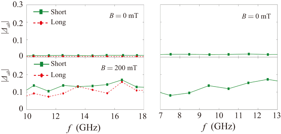
In Fig. 2 measured transmission spectra are exhibited for the MB1 with short and long antennas for B = 0 mT and B = 200 mT. To facilitate comparison with other spectra black dashed vertical lines are plotted at the positions of the resonances of the MB1 with short antennas. Their comparison with those obtained with long antennas shows that they induce a perturbation which is strong enough to shift the positions of the resonances, that is, the eigenfrequencies. This is confirmed by the spectral properties exhibited below. Also the effect of magnetization is that the resonances for B = 200 mT are shifted with respect to those for B = 0 mT, which also becomes visible in a change of the spectral properties. To estimate the size of T-invariance violation, we analyzed the violation of the principle of detailed balance, |S_ab| = |S_ba|, in terms of the measure^[70]Δ_ab = (||S_ab| – |S_ba||)/(|S_ab| + |S_ba|). Here we used the non-calibrated S-matrix elements, because at superconducting conditions a special procedure is required, which is cumbersome.^[109–112] Since we are only interested in spectral properties of the MBs, this procedure is not needed. Yet, we cannot get any information on the strength of T-invariance violation from phase-dependent fluctuation properties of the S matrix, like the cross-correlation coefficients.^[69,70] In Fig. 3Δ_ab is plotted for the MB1 (left) and the MB2 (right). For B = 0 mT the principle of detailed balance is fulfilled up to experimental accuracy, whereas for B = 200 mT its size is similar for MB1 with short antennas and MB2 and slightly smaller for MB1 with long antennas.

The RP model is a paradigmatic RMT model^[47] which is applied to characterize the spectral properties of typical quantum systems, whose classical counterpart exhibits a mixed integrable-chaotic dynamics. These are predicted to exhibit a behavior intermediate between Poisson and WD statistics. The model depends on a parameter λ which induces a transition from a random matrix which is diagonal to one from either of the WD ensembles, denoted as H^0 and H^β, respectively,

The probability density of the elements of H^0 is arbitrary. We chose them as Gaussian distributed random numbers, where the variance equals that of the diagonal elements of H^β, σd2=〈Hnn2〉=1/(2βN) and that of the off-diagonal elements of H^β is σoff2=〈(Hnm(q))2〉=1/(4βN). Here N denotes the dimension of H^ and q = 0,…,β–1 counts the number of independent components of the off-diagonal matrix elements of H^. For β = 1, H^0→β(λ) is real symmetric, whereas for β = 2 it is complex Hermitian. The scaling of λ, denoted by Γ_N is introduced to ensure that the spectral properties of the unfolded eigenvalues do not depend on the dimension of H^0→β(λ).^{[2,77,81,113,114]} We followed Ref. [114] and chose it equal to the inverse of the average density of the diagonal elements of H^0; see Eq. (1). With increasing λ the matrix elements of H^β become dominant, implicating a transition of the spectral properties from Poisson to WD statistics.

Recently, we studied the transition from Poisson to GUE experimentally with an MB.^[54] In this paper we analyze experimental data for cavities with the shapes of CBs whose dynamics is intermediate between integrable and chaotic and whose spectral properties agree with those of the RP model Eq. (1) with β = 1, subject to a non-vanishing external magnetic field applied to a ferrite which acts as a random potential and induces partial T-invariance violation. The objective is to verify, whether such systems, or generally, typical quantum systems with these features are described by an extended RP model comprising random matrices given by

where H^A is antisymmetric with Gaussian distributed random numbers with zero mean and the same variances σ_off, as in the RP model Eq. (1). Note, that equation (2) can be brought to the form

with η = λ + ξ. To determine the sizes of chaoticity and of T-invariance violation, we use the known Wigner-surmise like nearest-neighbor spacing distributions (NNSDs) for the RP model Eq. (1)^{[50,60,115,116]} and derive a corresponding analytical expression for the RP model Eq. (2), which is validated with the experimental data. These analytical results are employed to identify the RMT model suitable for the description of the experimental data and to determine the parameters λ,η,ξ entering Eqs. (1) and (2). Based on the thus determined parameters and the corresponding RP model we then compute other statistical measures for short- and long-range correlations.

In Appendix B we derive an analytical expression for the Wigner-surmise like NNSD of the extended RP model Eq. (2),

with

and D∼=D/(22η) with D=∫0∞dssP0→1→2(s;D∼=1/[22η]). As outlined in the Appendix B, in the limits ξ → 0 and ξ → η the results Eqs. (B1) and (B2) are recovered, respectively.

For the analysis of spectral properties the sorted eigenfrequencies f_n, f_n < f_n+1 are unfolded to average spacing unity by replacing them by the smooth part of the integrated resonance density Nsmooth(f), εn=Nsmooth(fn). For QBs and MBs with metallic walls it is given by Weyl’s formula

with A and L denoting the area and perimeter of the billiard, respectively, and it provides for B = 0 mT a good approximation for the cavities, which contain a ferrite disk instead of a metallic disk at the center. For B ≠ 0 mT, Nsmooth(f) is obtained by fitting a quadratic polynomial to the experimentally determined N(f). The parameters λ, ξ, η of the RP models Eqs. (1) and (2) were determined in all considered cases by fitting the corresponding Wigner-surmise like approximation to the experimentally determined NNSD. Note, that the sizes of T-invariance violation and chaoticity induced by the magnetized ferrite depend on frequency^[69,97,117] wherefore we analyzed spectra in frequency windows, whose widths were chosen such that the size of chaoticity and of T-invariance violation depend only weakly on frequency.

First, we applied the analytical result Eq. (3) for the NNSD of the RP model Eq. (2) to that of the eigenfrequencies of the MB1 with short antennas and B = 200 mT. The resulting curves are plotted as blue squares in the left part of Fig. 4. They are compared with those obtained from the fit of the NNSD of the RP model Eq. (1) with β = 2 (red dots); see Ref. [54]. Here, we divided the eigenfrequency spectrum into the frequency windows given in the legends of the panel. The crucial difference between the RP models Eqs. (1) and (2) is, that in the former model the size of chaoticity and T-invariance violation are characterized by one parameter ξ_L, whereas in the latter the effects inducing chaoticity and T-invariance violation are described by two independent parameters η and ξ. The very good agreement between the red and blue curves and of the parameter values implies that, as assumed in Ref. [54], indeed the chaoticity and T-invariance violation, that are induced by magnetizing the ferrite at the center of the cavity, are accounted for by one parameter ξ_L. This finding is confirmed in the right part of Fig. 4. There, we compare the experimental ratio distributions with the analytical Wigner-surmise like result for the RP model Eq. (1) for β = 2 given in Eq. (C1), which was derived by one of the authors (BD) in Ref. [95]. The parameters ξ_L resulting from the fit with Eq. (C1) to the experimental ratio distributions is similar to that obtained with Eq. (B2) for the NNSD and the agreement between theory and experiment is very good. We also show the experimental results for the eigenfrequency range 10 GHz–20 GHz. Using the whole frequency range is equivalent to superimposing spectra with different values of λ_L, ξ_L or η and ξ so that the fit yields averages over these parameters, as confirmed; see legends in the panels.

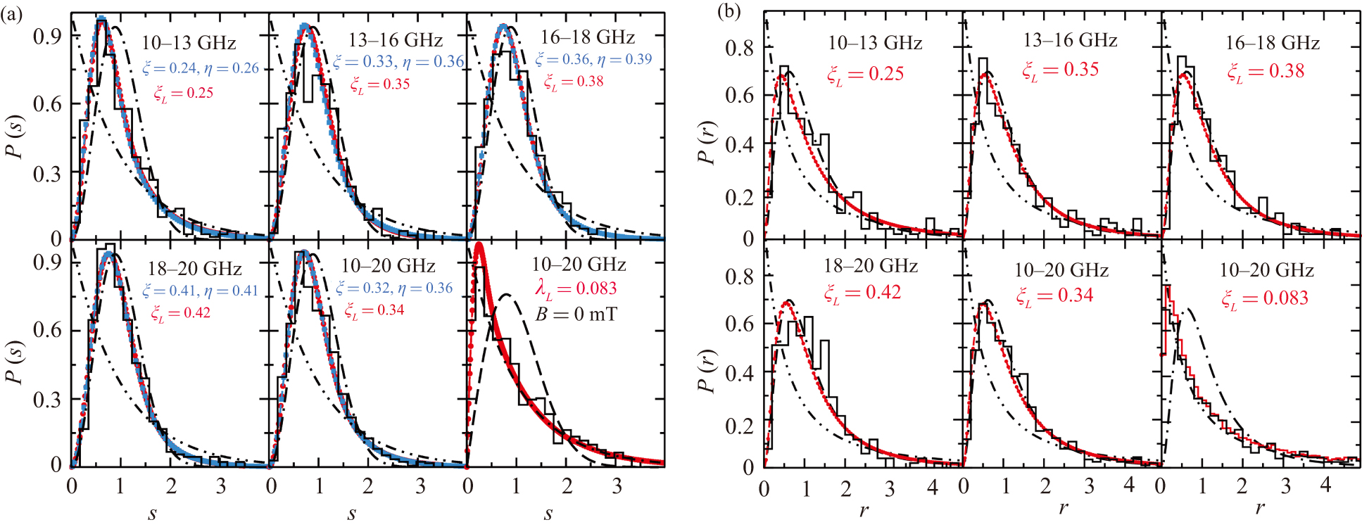
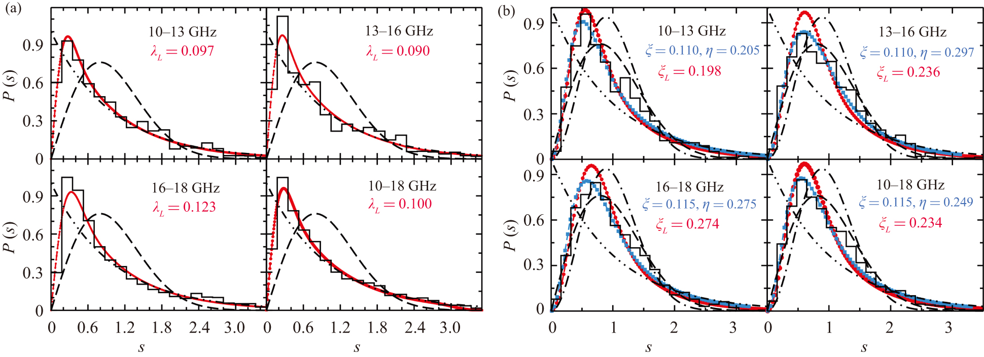
In Fig. 5 we compare the NNSDs obtained for the MB1 with 10 long antennas for B = 0 mT (left) and B = 200 mT (right) to the best fitting analytical curves obtained from Eq. (B1) (red dots in the left part), Eq. (B2) (red dots in the right part), and Eq. (3) (blue squares in the right part). Here, the spectra were divided into the frequency ranges comprising 257 eigenfrequencies. Note that similar to the singular MBs containing only one long antenna the size of the perturbation depends on the frequency. However, as indicated by the values of λ_L obtained from the fits, it seemingly barely changes in the frequency range from 10 GHz–16 GHz and differs only slightly from the one in the range from 16 GHz–18 GHz. These results imply, that indeed the spectral properties are intermediate between Poisson and GOE statistics for B = 0 mT, yet closer to Poisson than to WD statistics as confirmed by the comparatively small value of λ_L. This indicates that the classical dynamics is mixed regular-chaotic with a small chaotic component. As visible in the right figure, the best-fitting curves obtained with Eq. (B2) as fit function clearly differ from those obtained with Eq. (3). Furthermore, the agreement of the latter with the experimental curves is better than that for the former, as expected, because for B = 0 mT the dynamics is not fully integrable, as assumed in the RP model Eq. (1). The values of ξ_L are smaller than those for the measurements with short antennas, implying that T-invariance violation is weaker in that case, in agreement with Fig 3. To verify the applicability of the RP model Eq. (2) we performed the random-matrix simulations to compute other statistical measures, for which analytical results are not available. We inserted the parameter values resulting from the fit of Eq. (3) into that equation and analyzed the Dyson–Mehta statistics Δ₃(L), that is the spectral rigidity,^[8,118] which provides information on long-range correlations, and the distribution of ratios r_n = (f_n+1 – f_n)/(f_n–f_{n – 1}) of the non-unfolded eigenfrequencies.^[119–121] As illustrated in Fig. 6, for both statistical measures the agreement between the experimentally determined curves and those obtained from the ensemble average of 200 400 × 400-dimensional random matrices of the form Eq. (2) is good.

In the right figure we also show the curves computed from Eq. (C1) using the values of ξ_L obtained from the fit with Eq. (B2). In contrast to the NNSDs, the ratio distributions of the RP models (1) and (2) barely differ. This implies, that the NNSD is more sensitive to slight perturbations, i.e., in the present case to differences between η and ξ, than the ratio distribution, thus confirming the observations made in Ref. [95]. Consequently, the Wigner-surmise like NNSD is a more appropriate tool for the determination of the size of chaoticity and T invariance than the ratio distribution.

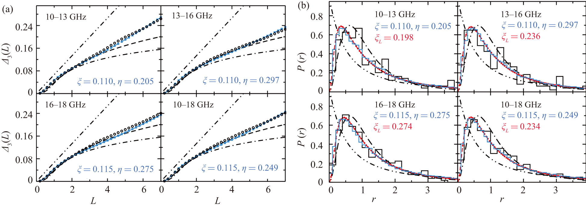
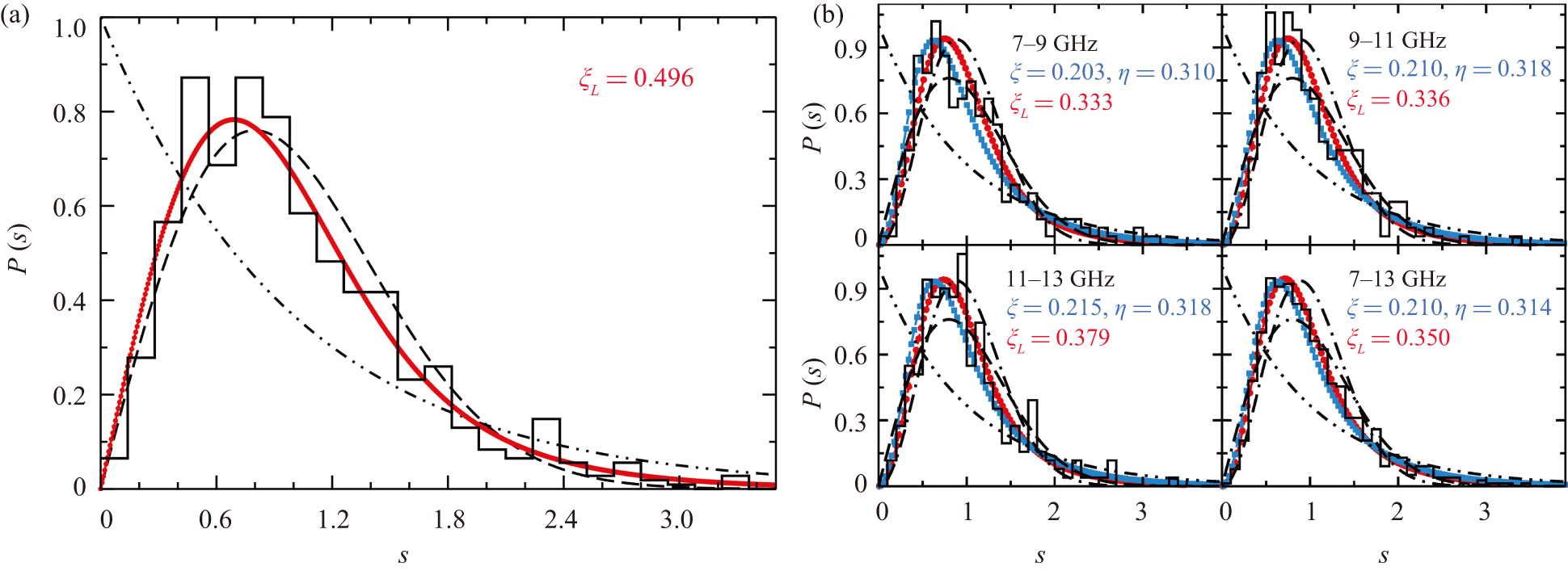
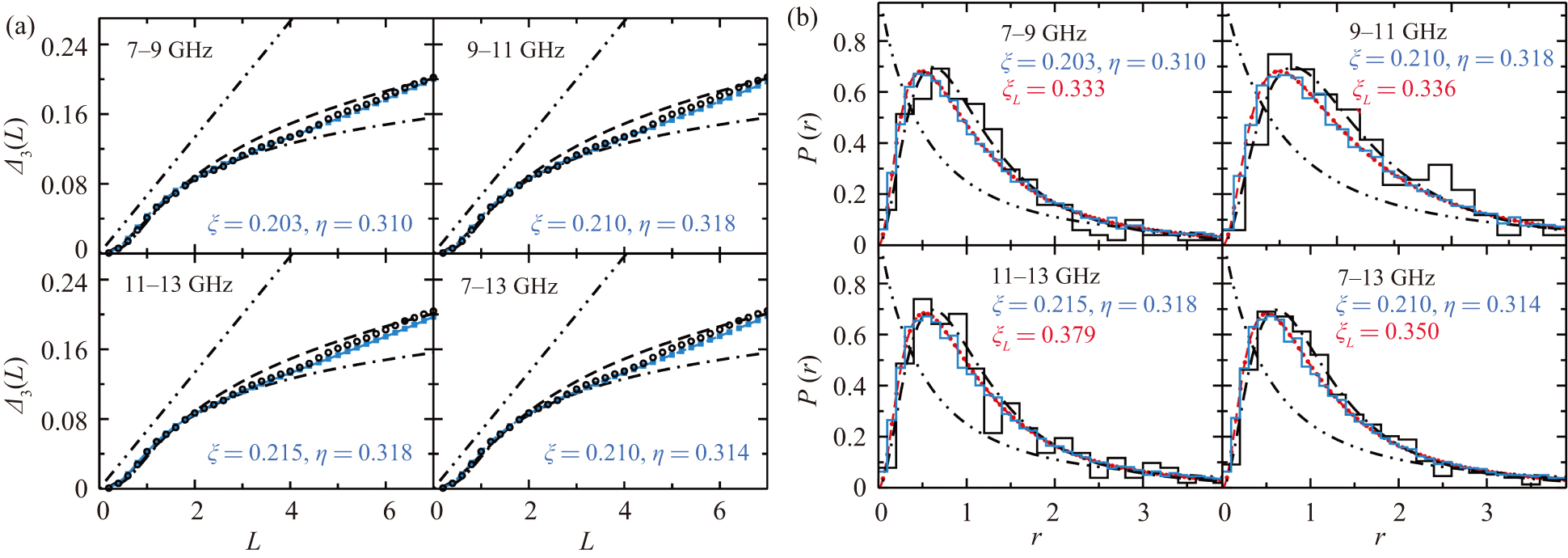
In Fig. 7 the NNSDs of the MB2 with B = 0 mT (left) and B = 200 mT (right) are exhibited. In this case the spectral properties are closer to WD statistics than to Poisson statistics in both cases. Furthermore, the curves obtained from Eq. (B2) (red dots) differ considerably from those deduced from Eq. (3) (blue squares), and the latter agree well with the experimental results. Note, that in this case the perturbation induced by the two scatterers is stronger than that due to the long antennas, so that the chaotic component is already large for B = 0 mT. The sizes of the parameter ξ_L are comparable to those for the MB1 with short antennas, thus confirming the results in Fig. 3. We again verify the applicability of the RP model Eq. (2) by performing random-matrix simulations. Comparing the Dyson–Mehta statistics and ratio distributions for the values of η and ξ obtained from the fits employing Eq. (3) to the corresponding experimental results yields a good agreement as demonstrated in Fig. 8. Similar to the results obtained for the MB1 with long antennas, the ratio distributions obtained with the RP model Eq. (1) are barely distinguishable from those resulting from the model Eq. (2), thus confirming our previous conclusion that they are not suitable for the determination of the size of chaoticity and T-invariance violation.

We propose a procedure to determine the size of chaoticity and T-invariance violation of typical quantum systems whose classical dynamics experiences a transition from mixed regular-chaotic to fully chaotic with complete T-invariance violation. It involves an extended RP model proposed in this paper and the Wigner-surmise like analytical result for the corresponding NNSD, whose derivation is provided in the appendix. This procedure is verified with experimental data obtained by inducing in MBs, whose top and bottom plates are made from niobium, a superconductor of type II,^[74] and whose spectral properties are between Poisson and GOE and well described by the RP model Eq. (1) with β = 1, T-invariance violation with a ferrite, that is magnetized with an external magnetic field B. The experiments were performed at superconducting conditions, thereby achieving high-quality factors even for nonzero magnetic field B, a prerequisite to facilitate the identification of a complete sequence of ∼1000 eigenfrequencies. Accordingly, we were able to analyze the spectral properties in various frequency ranges containing about 250 eigenfrequencies and to study the gradual transition from spectral statistics between Poisson and GOE to GUE. To validate the proposed procedure we computed for the thus determined parameter values long-range correlations, for which no analytical results are available, for the experimental data and the RMT model Eq. (2) and found good agreement between them. Furthermore, we experimentally verify with the data for the MB1 with short antennas an analytical expression for the ratio distribution of the RP model Eq. (1), derived by one of the co-authors in Ref. [95].

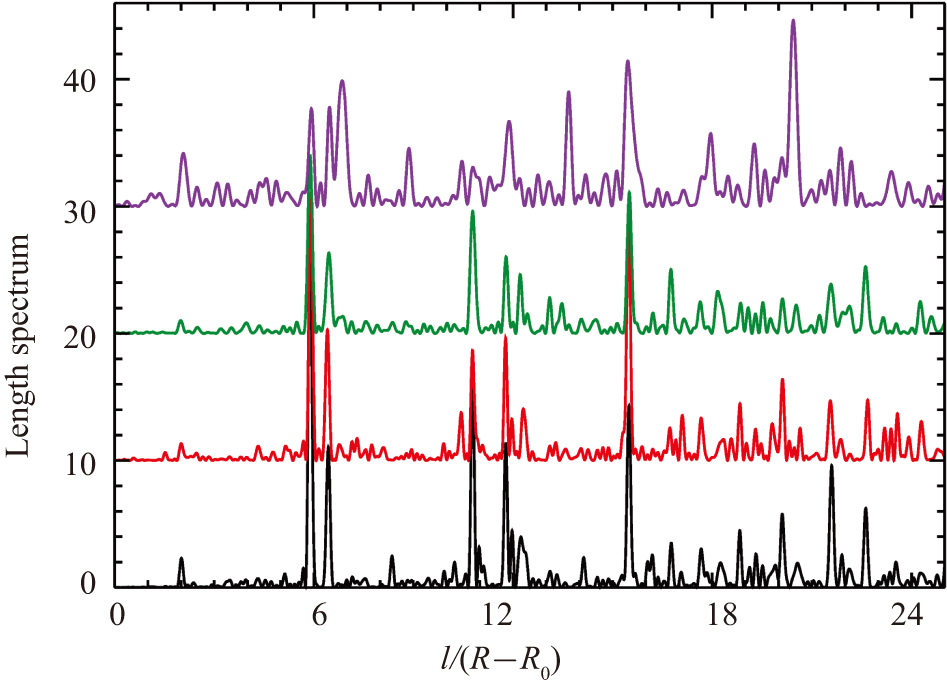
The modulus of the Fourier transform of the fluctuating part of the spectral density from wave number to length yields a length spectrum. It has this name because it exhibits peaks at the lengths of the periodic orbits of the corresponding classical system.

In Fig. A1 are exhibited from bottom to top the length spectra for the ring QB, for the MB1 with short and long antennas and for the MB2. The length spectra of the QB and MB1 with short antennas mainly differ at lengths that correspond to orbits that hit the inner billiard wall and the ferrite disk, respectively. This is attributed to the differing BCs at these walls, namely mixed Dirichlet and Neumann BCs for the MB, implying that there is no specular (hard-wall) reflection at the ferrite-disk wall in the ray-dynamical limit.^[54] The length spectrum for the MB1 with long antennas clearly differs from that with short antennas, as it shows additional peaks that may be attributed to orbits that hit the antennas.^{[107,122,123]}

The Wigner-surmise like approximations for the NNSD of random matrices from the WD ensembles and the RP model Eq. (1) have been derived based on 2 × 2-dimensional random matrices. For the case β = 1 in Eq. (1) it is given by^[50]

where D∼=D/(22λL) with

and I₀(x) is the modified Bessel function. The distribution experiences a transition from Poisson for λ_L = 0 to the Wigner surmise for β = 1 for λ_L → ∞. In Ref. [60] the corresponding Wigner-surmise like approximation was derived for the case β = 2 in Eq. (1),

where D∼=D/(22ξL) with

and z=pD∼s/2ξL. The proof that these distributions approach the corresponding WD surmise for λ_L → ∞ and ξ_L → ∞, respectively is straightforward. The Poisson distribution is recovered for λ_L → 0 and ξ_L → 0 employing that

where the limits have to be taken such that λ_L < s or ξ_L < s, respectively.

We verified the scaling of the parameters λ_L and ξ_L, which differ by a factor of 2 from those given in Refs. [50,60,103,115,116], by comparing P^{0 → β}(s;D) to ensemble averages of the NNSD of the eigenvalues of 200 N × N-dimensional random matrices with N = 400,800,1200 of the form H^0→β(λ) in Eq. (1). This yielded that the analytical and numerical distributions agree well for λ = λ_L and λ = ξ_L for β = 1 and β = 2, respectively. The discrepancy to previous results^{[50,54,60,95]} originates from the scaling Γ_N of λ introduced in Eq. (1).

Based on the joint probability distribution of the eigenvalues of H^0→2(λ) for the transition from Poisson to GUE^{[60,81,82,124]} one of the authors (BD) derived in Ref. [95] a Wigner-surmise like analytical expression for the ratio distribution,

where Xi=Ai(φ)/Fi(φ), i = 1,2 with

and R = (2/3)(1+r+r²). It is proven there that

which is the ratio distribution for the eigenvalues of a 3 × 3-dimensional diagonal matrix with Gaussian distributed entries, and

which is the ratio distribution for the Wigner-surmise like analytical result for the GUE. Note, that in the derivation the matrix elements of the diagonal matrix H₀ in Eq. (1) were chosen as Gaussian distributed matrix elements, as in the numerical simulations; see below Eq. (1). More information can be found in Ref. [95].

A Wigner-surmise like expression for the NNSD of random matrix describing the transition from Poisson to GOE and then to GUE, experienced when exposing it to T-invariance violation, is obtained based on 2 × 2 random matrices of the form Eq. (2),

with η∼=2η, ξ∼=2ξ, A = ηh₁₁, B = B₁ + iB₂ where B1=η∼h12, B2=ξ∼ε, and C = p + ηh₂₂. Here, the factor 2 accounts for the scaling Γ_N in Eq. (2), for which the parameters λ_L, ξ_L, η, ξ measure the size of the parameters in units of the inverse of the average density of the entries of H₀. Furthermore, we transformed the matrix H₀, whose elements p₁,p₂ are uncorrelated random numbers, to one which only depends on the non-negative spacing p between them.^[116] Its probability density is given as P₀(p) = e^−p. Furthermore, h₁₁, h₂₂, and h₁₂, ε are Gaussian-distributed random numbers with zero mean and variance 1 and 1/2, respectively, yielding for the distributions of A, B, and C

where we introduced σ₂ = 2η², σ₃ = 2ξ². Then the NNSD P^{0 → 1 → 2}(s) is obtained by computing the ensemble averages of the matrix elements of random matrices under the condition that the spacing of the eigenvalues

of H^0→1→2 is s=(A−C)2+4|B|2,

To perform the integrals over B₁ and B₂ we introduce polar coordinates, B₁ = ρcosϕ, B₂ = ρsinϕ and obtain for the integrals in Eq. (D4)

with

Next, we introduce the variable A∼=(A−C) and perform the integral over C yielding

Rescaling to average spacing unity yields the distribution Eq. (3),

with D∼=D/(22η), where

In the limit ξ → η, that is, Σ → 1 and Δ → 0 I0((D∼s)2Δ(1−x2))→Δ→01 so the integral over x can be performed and the result for P^{0 → 2}(s) in Eq. (D2 is recovered. For ξ → 0 the integral (D5 becomes with the notation x = (A–C)/s

yielding

which turns into the results for the transition from Poisson to GOE after rescaling the spacings s to mean spacing unity.