Observation of Weibel magnetic fields in laser-produced interpenetrating flows

Weibel instability (WI) is an electromagnetic instability which occurs frequently in interpenetration processes, such as the ejection of material from supernova,^[1–4] the interaction between solar wind and interstellar media,^[5] gamma ray bursts,^[1,6] jets,^[7,8] and the accretion from massive astrophysical objects.^[9] The study of WI is significant to understand astronomical phenomena associated with physical processes in the universe, such as collsionless shock formation, magnetic field generation and amplification, particle acceleration, and so on.

The use of laboratory laser facilities provides a new way to study the details of the WI in interpenetrating plasma flows.^[10,11] There are two methods of generation of interpenetrating plasma flows in laboratory.^[12] One is ablating a foil with laser beams, which results in the generation of a reverse flow from the opposing foil due to the scattering of lasers and x-rays from the laser-ablated target.^[13–16] The other one is employing two bunches of laser beams, which are used to ablate the facing surfaces of two foils and directly generate the interpenetrating plasma flows.^[17,18] Over the past twenty years, significant progresses have been made in the laboratory study of WI. For instance, Weibel-mediated-shock formation^[19] and the magnetic field amplification,^[18,19] and a recent study revealing that WI can mediate kinetic turbulence formation, where the electrons gain energy via stochastic acceleration process.^[20]

It is well known that the linear growth rate of WI is proportional to v⋅ne1/2, where v is flow velocity and n_e is electron density.^[20] Previous studies have demonstrated the WI in linear phase with typical flow velocity v ∼ 1 × 10⁸ cm⋅s⁻¹ and electron density n_e ∼ 5 × 10¹⁸ cm⁻³. The corresponding linear growing time is about 5 ns.^[18,19] In this paper, we mainly focus on the nonlinear WI by enhancing flow velocity and electron density, v ∼ 2 × 10⁸ cm⋅s⁻¹ and n_e ∼ 1.2 × 10¹⁹ cm⁻³, whose linear growth time has been reduced as 224 ps. The maximum value of average magnetic strength is approximately 40 T.

Our experiment is performed at Shenguang-II laser facility in Shanghai, China. The overall experimental layout is shown in Fig. 1.

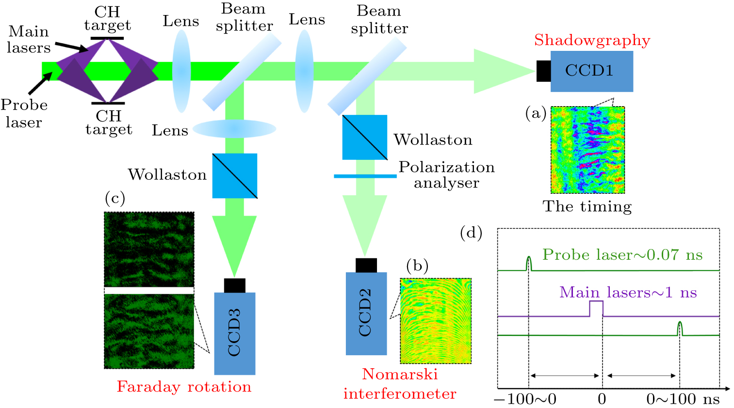
All eight main beams, with an energy of 230 J/beam, a wavelength of 351 nm (3ω) and a pulse width of 1 ns, are symmetrically focused on a pair of opposing CH–CH foils at the same time. The focal spot has a diameter of 150 μm, and the intensity is approximately ∼ 10¹⁵ W⋅cm⁻². Each foil has dimensions of 2 mm×2 mm×200 μm and the foils are separated by 4.2 mm. A linearly polarized laser, with a wavelength of 527 nm (2ω) and a pulse width of 0.07 ns, transversely passing the interaction region, is used as probe for optical diagnostics. As shown in Fig. 1(d), by adjusting the time interval between the probe and the main lasers, we can observe the evolution of interpenetrating plasma.

The linearly polarized probe is split into three beams. One beam enters the shadowgraphy channel, which is used to observe the profile of the plasma, as shown in Fig. 1(a). The probe passes through the plasma and is refracted due to the density gradient within the plasma, the profile of the plasma can be observed at the image plane. Imaging magnification is 1.10 for the shadowgraphy channel. The second beam enters the Nomarski interferometer channel, which is used for the inference of the plasma density, as shown in Fig. 1(b). The probe passes through the Wollaston prism and is split into two beams with perpendicular polarization directions. The two beams then pass through the polarization analyzer and interfere with each other at the image plane. In order to measure the plasma density, we first need to obtain reference image without plasmas. After that, we can obtain a raw image at different time when the plasma is present. By comparing the two images, we can infer the density of the plasma from the shifted fringes. Imaging magnification is 1.44 for the Nomarski interferometer channel. Finally, the third beam enters the Faraday rotation channel, which is used to infer the longitudinal (parallel to the direction of the probe) magnetic strength of the plasma, as shown in Fig. 1(c). The probe passes through the Wollaston prism and is split into two beams. Different polarization directions of probe can result in varying light intensities at the image plane. As mentioned above, in order to obtain the longitudinal magnetic strength, we need to compare the images with and without plasma, which will also result in a change to the polarization direction. The path integral of the magnetic strength ∫0Lne′Bdl can be determined by analyzing the change in intensity of the probe. Here, ne′ is the electron density of interaction region, B is the magnetic strength, L is the length of the path of the probe through the plasma. Imaging magnification is 2.84 for the Faraday rotation channel. The temporal-spatial resolution of our optical diagnostics is about 100 ps and 20 μm.

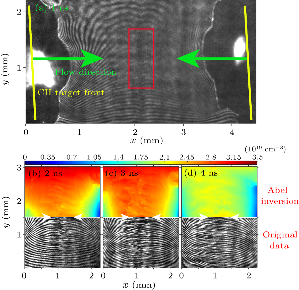
The whole evolution of interpenetrating flows is obtained by Nomarski interferometer, where the shifted fringes in the image represent the presence of plasma. As shown in Fig. 2(a), the interference fringes in the middle (marked by red rectangular box) have bent at 1 ns. It means that the two interpenetrating plasma flows have formed and interacted with each other in the middle plane. This fact also indicates that the corresponding mean relative velocity in 0–1 ns of the two plasma flows is v_rel = L/t ∼ 4 × 10⁸ cm⋅s⁻¹. However, the plasma density is hard obtained at 1 ns due to the missing fringes. Therefore, we use half of the interpenetrating region plasma density to represent one side plasma flow density, as shown in Figs. 2(b)–2(d), we can find that the electron density within the interpenetrating region keep on order of ne′∼1019 cm⁻³.

The topology and corresponding path integral of magnetic strength ∫0Lne′Bdl can be obtained by Faraday rotation, as shown in Fig. 3. For the topology, at 1 ns, there is no filamentary structures in field of the view, because the two plasma flows have just met. At 2 ns, the filamentary structures appear in the middle plane when both plasma flows interpenetrated with each other. The filamentary region length is about 0.5 mm (1.25 mm < x < 1.75 mm). At 3 ns, the filaments and filamentary region length become longer, the filamentary region length is about 0.9 mm (0.8 mm < x < 1.7 mm). At 4 ns, the filaments are thickened, the filamentary region length increases to 1 mm (0.75 mm < x < 1.75 mm). It is worth noting that the observed structure of filament is three-dimensional (3D) in practical situations. In our experiments, the optical image is two-dimensional (2D), which leads to some filaments overlapping and makes us overestimate the length and thickness of some filaments. And the projection also makes us underestimate the distance between two filaments in 2D image. Some references also call this 3D effect as “forest effect”.^[19,21] Here we assume that all estimated values are reasonable (at least on the same order), because the probability of multiple filaments overlapping is low, the average distance between two filaments in 2D image and in 3D space only differ by a factor ∼ cos 45°.

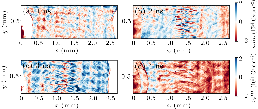
For the path integral of magnetic strength, at 1 ns, there is no strong magnetic field area in the background magnetic field. At 2 ns, there is a strong magnetic field area in the middle plane with filamentary structures. The average path integral of the magnetic strength is about ∫0Lne′Bdl=1.6×1024 Gs⋅cm⁻² (1 Gs = 10⁻⁴ T). Taking the measured electron density ne′=2.8×1019 cm⁻³ (as shown in Fig. 2(b)) and assuming the length of the path equal to target size L = 2 mm (the same below), the strength of magnetic fields can be inferred as 28.6 T. At 3 ns, the average path integral of the magnetic strength is about ∫0Lne′Bdl=2.0×1024 Gs⋅cm⁻². Taking the measured electron density ne′=2.8×1019 cm⁻³ (as shown in Fig. 2(c)), the strength of magnetic fields can be inferred as 35.7 T. At 4 ns, the average path integral of the magnetic strength is about ∫0Lne′Bdl=1.6×1024 Gs⋅cm⁻². Taking the measured electron density ne′=2.0×1019 cm⁻³ (as shown in Fig. 2(d)), the strength of magnetic fields can be inferred as 40.0 T.

The mean free path (MFP) is a key parameter in determining whether the interaction between interpenetrating plasma flows is collisionless. The ions MFP λ_ii (International System of Units) can be expressed as λii=2πε02mi2vrel4/(niZ4e4lnΛ)^[22] (here we ignore the thermal velocity), where ε₀ is the vacuum permittivity, m_i is the average ion mass (m_i = Am_p, A = 6.5 is the average mass number and m_p is the proton mass), v_rel is the relative velocity (we take v_rel = 4 × 10⁶ m⋅s⁻¹, which is obtained in Fig. 2), Z is the average degree of ionization (Z = 3.5, we assume that carbon and hydrogen are completely ionized under the intensity approximately 5 × 10¹⁵ W⋅cm⁻²), n_i is the ion density (n_i = n_e/Z, we take n_e = 1.2 × 10¹⁹ cm⁻³), e is the elementary charge and ln Λ is the Coulomb logarithm. The Coulomb logarithm can be expressed as lnΛ=ln(4πε0λDmrvrel2/(Z2e2)), where λ_D is the Debye length, and m_r = (1/m_left + 1/m_right)⁻¹ = m_i/2 is the reduced mass, where m_left and m_right are the average ion mass coming from the left and right plasma flows. Additionally, one can find that the value of Coulomb logarithm is insensitive to the plasma temperature. Here we use temperature kT_e is roughly estimated as 1 eV–1000 eV, we obtained ln Λ ∼ 11.1–14.6, the corresponding MFP is 3.0 m–4.0 m, still much smaller than the distance of two targets (4.2 mm). This value strongly indicate that the interaction between interpenetrating plasma flows is collisionless.

It is well known that there are two types of instability occuring in interpenetrating plasma flows. One is the electrostatic instability, also known as the two-stream instability. Electrostatic instability is caused by spatial density perturbation of electrons and ions, which is due to the excessive temperature difference between the two kinds of particles. The typical space value induced by electrostatic instability is on order of c/ω_pe and the corresponding time scale is 1000 < ω_pet < 5000, where ω_pe is the electron plasma frequency.^[23] Taking our experimental parameters into above expressions, we can obtain that the filament spacing is about 1.5 μm and time scale for the existence of filaments is 5.1 ps–25.6 ps, much smaller than our experiment diagnostic resolution. So the filaments induced by electrostatic instability can be ruled out in our experiments.

The other one is Weibel-type instability, which can be induced by temperature anisotropy or velocity anisotropy. In the linear phase, the width of filaments almost keeps constant and the length of filaments elongates along the flow direction, the magnetic strength increases exponentially due to a positive feedback loop, which means that the net current generates magnetic field and the magnetic field serves to further constrain the current. After entering the nonlinear saturation phase, the width of filaments becomes thicker via magnetic reconnection process,^[24] while the magnetic strength reaching saturation state is roughly constant if the plasma conditions are homogenous and constant.^[21,25] Here the linear growth rate of WI can be expressed as Γ ∼ 0.1 × v_relω_pi/c,^[20] where ω_pi is the ion plasma frequency, the corresponding linear growth time can be expressed as t = 1/Γ ∼ 224 ps, indicating that WI will quickly entered nonlinear phase after both flow interactions ∼ 224 ps. It indicates that the observed filaments in our experiment (Figs. 4(b)–4(d)) have entered the nonlinear saturation phase. The filamentary region length can be estimated as l_EM ∼ Kc/ω_pi, where K = 10 is a typical numerical factor representing the growth times of the WI, c/ω_pi is the ion plasma skin depth.^[26] One can obtain that the theoretical filamentary region length l_EM = 0.9 mm is consistent with this experimental results. From the measured Weibel magnetic field, we can find that the strength quickly increase about 28.6 T from 1 ns to 2 ns. After that, the magnetic strength increases slowly from 28.6 T to 40 T from 2 ns to 4 ns, indicating that WI has entered the nonlinear phase and finally reached saturation. All the characteristics are consistent with the theory of WI evolution.

To support our experimental results, scaled-down 2D particle-in-cell (PIC) simulations of WI are performed with the OSIRIS codes.^[27] The simulation box of 4000 μm (x) × 400 μm (y) with 16 macroparticles in each cell is conducted with high longitudinal and transverse resolutions of Δx = 1/12 μm and Δy = 1/16 μm. The initial value of the electromagnetic fields is set to zero and m_i/m_e = 1836, where m_e is electron mass. A flow velocity v_sim = 3 × 10⁹ cm⋅s⁻¹ and electron density n_sim = 5 × 10²⁰ cm⁻³ are used in order to reduce the computational load. This treatment allows us to simulate the WI process matching the experimental case with a reduced time scale.

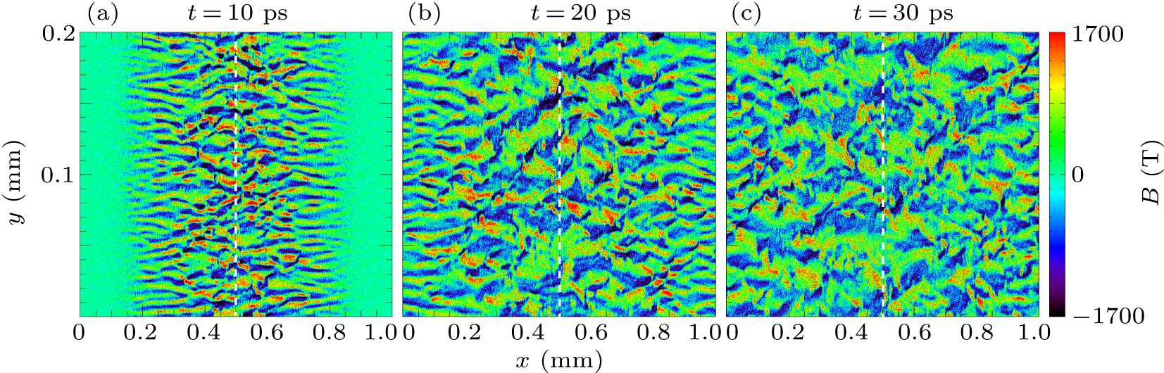
As shown in Fig. 4, two plasma flows are come from the left and right sides (±x) of the box. At t = 0 (corresponding to 1 ns in experiment), two plasma flows meet each other at the midplane. Then the WI begins to grow, filamentary structures appear. As shown in Fig. 4(a), filamentary region length is about 0.6 mm. The length and width of filaments are about 0.1 mm and 5 μm. The magnetic strength is about 1700 T. As shown in Figs. 4(b) and 4(c), the filamentary region length expand to both sides. The length and width of filaments become longer and thicker with the growth of WI. The magnetic strength increases slowly. All features of the nonlinear WI are consistent with the experiment results.

Under scaling laws,^[28] one can obtain that the relationships of time, magnetic strength and length between simulation and experiment are t_sim/(t – 1 ns) ∼ 1/100, B_sim/B ∼ 100, and x_sim/x ∼ 1/6.5, the constant 1 ns is due to the fact that the moment when two plasma flows meet is 1 ns in the experiment. Some important parameters and the results of scaling transformation are shown in Table 1.

It can be observed that if we convert the simulated magnetic strength and length into experiments, the magnetic strength ∼ 17 T is lower than the experimental value, and the length ∼ 6.5 mm is greater than the experimental value. This may be due to the fact that the plasma flow generated in our experiment does not have a uniform density distribution, while the plasma flow used in the simulation has a uniform density. We need to know that the density in the central region of the plasma flow is higher than that in the edge region in 3D situation. But we take an average value n_e = 1.2 × 10¹⁹ cm⁻³ for scaling transformation, i.e., B = B_sim⋅(v/v_sim)⋅(n_e/n_sim)^1/2.^[28] Therefore, for higher density in the central region of plasma flow, the magnetic strength is relatively low after scaling transformation. The reason for the larger filamentary region length after scaling transformation is the same as above, i.e., x = x_sim⋅(n_sim/n_e)^1/2.^[28] In addition, as shown in Fig. 2(a), the plasma flows have already met at 1 ns. The velocity v = 2 × 10⁸ cm⋅s⁻¹ we took is lower than actual velocity. This also leads to the magnetic strength relatively lower after scaling transformation.

We believe that the filamentary structures induced by the nonlinear WI have been observed in our experiments. The amplifications of the Weibel magnetic field are measured about 40 T. While Weibel-mediated-shock is not observed in our experiments, it is due to the fact that the interaction region size much smaller than the necessary size for the collisionless shock formation. According to the recent numerical simulations, l_EM ∼ 300c/ω_pi is needed for collisionless shock formation,^[26] the corresponding interaction region l_EM = 300c/ω_pi = 26.9 mm much larger than our target size. Our further experiments will plan to increase the target size to produce the astrophysical collisionelss shock at higher-energy laser facility, for example, SG-II UP.^[29]